Conception, Construction and Evaluation of a Raspberry Pi Cluster

The goal of this work is to create an affordable, energy efficient and portable mini-supercomputer. Ideally, a cluster computer with little or no carbon footprint, individual elements that are inexpensive to replace, and a portable system that can be easily disassembled and reassembled.
Introduction
Raspberry Pis are revolutionizing the computer industry. Originally developed to provide low-cost computers to schools, they are expanding far beyond their intended use. This inexpensive technology can be used to accomplish previously unexplored tasks. One such technology is a cluster computer that can run parallel jobs. Many systems built for parallel computing tasks are either expensive or unavailable outside of academia. Supercomputers are expensive to purchase as well as to use, power, and maintain. Although average desktop computers have come down in price, the cost can still become quite high if they require a larger amount of computing power. In today's world of information technology (IT), it is not new to be confronted daily with new technologies such as cloud computing, cluster computing or high-performance computing. All these terms are approaches that are intended to simplify people's work and lives. Cloud providers such as Microsoft or Amazon make these types of technologies available to customers in the form of services for a fee. Users thus have the opportunity to use the computing power of these technologies without having to buy them at a high price. The advantage here is the almost unlimited scaling of resources. Distributed computing, an infrastructure technology and basis for the provision of cluster computers via the Internet, is used to meet increasing resource demands. By interconnecting and adding remote systems, computing power and performance can be dynamically scaled and provided in theoretically unlimited quantities.
Motivation and objective of the work
Unlimited computing power implies the solution approach to be able to solve seemingly unsolvable and complex problems, such as the simulation of black holes or the calculation of the Milky Way. Expensive supercomputers are oversized when it comes to testing new applications for high-performance computers or solving complex problems. In this work, we address the question of whether we can create an independent and comparable but also less expensive system with few resources, which allows us to solve complex problems in the same way. 24 years ago, Donald Becker and Thomas Sterling started the Beowulf project to create a low-cost alternative but also a powerful alternative to supercomputers. Based on this example, the idea has arisen to pursue the same principle on a smaller scale. The goal of this work is to create an affordable, energy efficient and portable mini-supercomputer. Ideally, a cluster computer with little or no carbon footprint, individual elements that are inexpensive to replace, and a portable system that can be easily disassembled and reassembled. A Raspberry Pi is ideal for this purpose because of its low price, low power consumption, and small size. At the same time, it still offers decent performance, especially when you consider the computing power offered per watt.
Procedure
This paper is divided into 5 parts. The first part is dedicated to the terminological clarification of background information on all technologies involved and how they are related to the cluster. Based on this, the second part clarifies the conceptualization, design, and requirements placed on the system. The main part deals with the construction of the Raspberry Pi cluster and thus forms the practical component, in which design decisions are illustrated and the construction is explained. Following this, important factors such as scalability, performance, cost and energy efficiency are discussed and evaluated. Different use cases are addressed and the technical possibilities are considered. Finally, evaluated evaluations are summarized, limitations are pointed out and future extensions are presented.
Background
This chapter covers the basic technologies that form the basis of parallel and distributed systems. These technologies build on each other, as in a layer system, and are dependent on each other. Architectures and techniques based on this, such as virtualization or cluster computing, in turn provide the basic framework for container virtualization and its management systems.
Parallel and distributed systems
Until computers evolved into distributed computing systems, there have been fundamental changes in various computing technologies over the past decades, which we will briefly discuss in order to make the basic framework of parallel and distributed systems more understandable.
Amdahl's and Gustafson's law
At the beginning of this work, the theoretically unlimited increase of computing power was mentioned. Amdahl's law (named in 1967 after Gene Amdahl) deals exactly with this question, namely whether an unlimited increase in speed can be achieved with an increasing number of processors. It describes, how the parallelization of a software affects the acceleration of this. One divides thereby the software into not parallel, thus sequentially executable and parallel executable portions. Sequential parts are process initializations, communication and the memory management. These parts are necessary for the synchronization of the parallel parts. They form dependencies among themselves and are therefore not able to be executed in parallel. Parallel executable parts are the processors, which are used for computation. It is very important to estimate how much performance gain is achieved by adding a certain number of processing units in parallel working system. Sometimes it happens that adding a larger number of computing units does not necessarily improve the performance, because the expected performance tends to decrease or oversaturate if we blindly add more computing resources. Therefore, it is very important to have a rough estimate of the optimized number of resources to use. Suppose a hypothetical system has only one processor with a normalized runtime of $1$. Now we consider how much time the program needs in the parallelizable portion and denote this portion by $P$. The runtime of the sequential part is thus $(1 - P)$.
The runtime of the sequential part does not change, but the parallelizable part is optimally distributed to all processors and therefore runs N times as fast. This results in the following runtime formula: 1
$$\underset{\text{sequential}}{\overset{(1 - P)}{︸}} + \underset{\text{parallel}}{\overset{\frac{P}{N}}{︸}}$$
This is where the time gain comes from:
$$Time\ gain\ according\ to\ Amdahl$$ $$= \ \frac{original\ duration}{\text{new\ duration}}$$ $$= \frac{1}{(1 - P) + \frac{P}{N}}$$
Here N is the number of processors and P the runtime portion of the parallelizable program. Gene Amdahl called the time or also speed gain Speedup. With the help of a massive parallelism the time of the parallelizable portion can be reduced arbitrarily, the sequential portion remains unaffected thereby however. As the number of processors increases, the communication overhead between the processors also increases, so that above a certain number, they tend to be busy communicating rather than processing the problem. This reduces the performance and refers to this as an overhead in the task distribution. A program cannot be completely parallelized, so that all processors are always busy with work at the same time. No matter how many processor units are used and the proportion of applications that cannot be parallelized is, for example, one percent, the speedup can be a maximum of 100. Gene Amdahl thus concluded that it makes no sense to keep increasing the computing units in order to generate unlimited computing power. 2
Amdahl's model remains valid until the total number of computing operations remains the same while the number of computing units continues to increase. However, if in our hypothetical simulation the job size increases while the number of computational units continues to increase, then Gustafson's law must be invoked. John Gustafson established this law in 1988, which states that as long as the problem being addressed is large enough it can be efficiently parallelized. Unlike Amdahl, Gustafson shows that massive parallelization is nevertheless worthwhile. A parallel system cannot become arbitrarily fast, but it can solve arbitrarily large problems in the same amount of time. 3
Client-server model
Client-server models are the basic techniques for operating distributed systems. They describe the principle of how tasks and services, such as sending e-mail or providing web applications, are distributed within a network. The corresponding service is centralized on a specific computer, called a server, and the other machines (clients) can use this service. 4
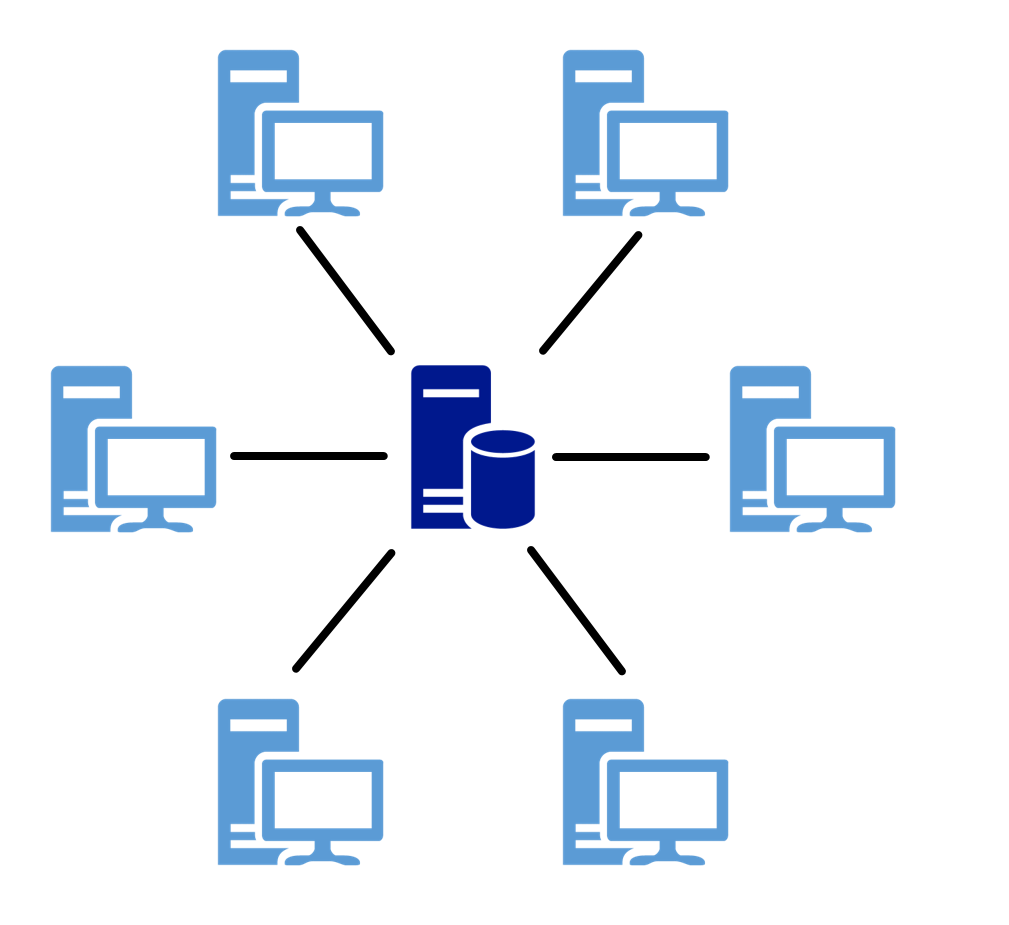
Figure 1: Illustration of the client-server model.
Operating systems (OS) such as Red Hat Enterprise Linux or Windows Server use the above concept and thus provide a client-server system. This is done by establishing the connection to the server on the client side and providing access to services and resources on the server side. Within these operating systems servers are simple programs, which are usually started automatically and run passively in the background. In the Linux environment these programs are called "daemon", under Windows Server they are called "service". In practice, however, different types of these server services are usually encountered. Examples of this are: 5
- Mail server: Communication service for electronic mail (e-mail).
- Web server: Transmitting web pages to clients.
- File server: A file server makes files available on a network.
Peer-to-peer
Peer-to-peer (P2P) systems are the opposite of client-server systems. In client-server networks, a server is not necessarily a specific computer. Server and client are referred to as roles in this context, since a computer can also act as a server and a client at the same time. In a P2P system, this distribution of roles does not exist; all computers have equal rights. A computer in a network is a peer because it can be a client and a server at the same time. It can both use and provide services. The functionality, the provision of a service, is therefore provided decentrally in a P2P system. 6
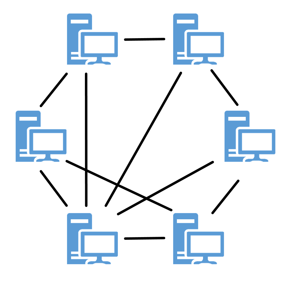
Figure 2: Illustration of the peer-to-peer model.
In contrast to the client-server concept, parallel and distributed systems are not based on P2P systems, but they have been part of the development process of grid and distributed computing and are therefore worth mentioning. 7
Grid Computing
The volume of data records in databases is increasing and will continue to increase in the coming years. Cluster systems (see Cluster) were developed to handle the complex processing involved and have since become established. However, the demand for computing power and storage capacity is becoming ever greater, especially in scientific areas such as medicine and research or in commercial areas such as e-commerce or financial management. Due to global networking of scientific working methods and international cooperation, more and more information technologies and infrastructures are being interconnected to create collaborative working environments. 8
Grid computing is a distributed computing technique that aims to connect loosely coupled computers and clusters and combine the computing power of all distributed resources into a virtual supercomputer. The basis for integrating these location-independent, cross-institutional, and autonomous resources is the use of existing network infrastructures such as the Internet. The major advantage over cluster systems is the aggregation and sharing of resources such as computers or databases across geographical boundaries. 9
Grid computing can be divided into the following classifications:
- Computing Grid: access to distributed computing resources.
- Data Grid: Access to distributed data volumes and storage capacity.
- Service Grid: Access to distributed applications and services.
A computing grid is comparable to a power grid. For the consumer, everything that happens behind a socket is hidden, but he can conveniently use the power offered, the electricity. A computing grid is similar in comparison, it connects to the computing network and uses the computing power offered. High costs or lack of financial resources pose solving complex problems as a difficulty for scientific and economic institutions. But due to the possibility like, the bundling of resources of different organizations, it is possible to solve computationally intensive problems cost-efficiently. 10
Public Resource Computing
As an analogous counterpart to grid computing, public resource computing (PRC) and volunteer computing have emerged to harness hidden computing power using distributed computing.
The idea and background of this type of distributed computing are that the use of supercomputers is very cost-intensive, on the other hand processors of many computers, such as those of personal computers (PC), servers or smartphones are not fully utilized. Many users work on their PCs with programs that use only part of the total processor power. To make these unused computing resources usable, a corresponding software client is installed on the respective PCs or servers, which establishes the connection to a computing grid, takes over task distribution and makes unused computing power available. 11
The software platform Berkeley Open Infrastructure for Network Computing (BOINC) enables the use of this unused computing power of thousands of computers. Examples of computationally intensive PRC projects and complex problems include creating an accurate three-dimensional (3D) model of the Milky Way, searching for extraterrestrial radio waves, and calculating gravitational waves. An example of a special research project that exploits the benefits of grid computing, and can only be realized using it, is grid-based computer simulations of gravitational waves generated by the merger of two singularities (black holes) (see Figure 3). 12
Other well-known RPC projects using BOINC are: 13
- SETI @home (Search for Extra-Terrestrial Intelligence at home): study of radio signal data from the Arecibo Observatory radio telescope in Puerto Rico used as evidence of extraterrestrial technology.
- MilkyWay@home: research in modeling and determining the evolution of the Milky Way Galaxy.
- Einstein@home: The project examines data collected by the LIGO and GEO600 gravitational wave detectors for evidence of periodic sources, such as rapidly rotating neutron stars, which are the gravitational equivalent of pulsars (pulsating radio sources).

Figure 3: Grid-based simulation of gravitational waves generated by the merger of two black holes.
It is worth mentioning the successes and cost savings achieved through the use of public resource or volunteer computing. Certainly it is possible to solve complex problems through high performance and supercomputers but not with such a small part of costs. For example, the University of Westminster, based in London, has been able to show savings of around £500,000 by using a BOINC supercomputer. 14
Distributed Computing
Distributed computing or distributed systems, as defined by Andrew S. Tanenbaum, is a collection of independent computers that appear to their users as a single unified system. Distributed computing resource processing deals with the coordination of these distributed computers. In contrast to cluster systems, most computers have different hardware and operating systems. In some cases, resources and programming languages vary greatly. The basic requirement for these machines to work together and exchange data is that they are connected via a network. 15
The computing technologies mentioned so far fall under the umbrella term distributed computing. Figure 4 shows how these technologies are classified collectively into distributed computing and, among others, into client-server computing and peer-to-peer.
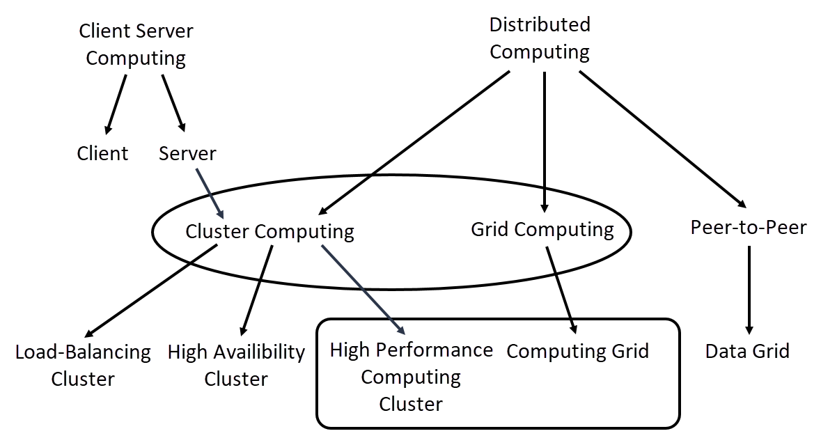
Figure 4: Schematic representation of computing technologies.
Communication networks such as the Internet form the basis for distributed systems and give the opportunity to connect geographically distant computers. The following prerequisites must be observed to prevent problems: 16
- Concurrency: Concurrency in the execution of programs must be ensured. As soon as services and applications are executed in a network of computers, this usually happens at different times and independently of other computers. To ensure this concurrency of applications, it must be possible to scale the system, which means that additional computers can be added to the network as the demand for resources increases.
- Time synchronization: As soon as systems act together, messages must be exchanged so that appropriate coordination is possible. Messages such as "System A is performing this action" and "System B is performing this action". For proper coordination of these messages, timestamps are needed to enable proper sequencing of these messages within the distributed system. One method of synchronizing system time is to synchronize with external atomic clocks outside of distributed systems or to use a shared time server that uses the Network Time Protocol (NTP), a standard protocol for synchronizing clocks on the Internet.
- Partial failure: Any system, no matter how well secured, can fail, even if it has an availability of 99.9%. The probability of a failure is still 0.1%, which is already a very large amount for a high number of systems. Care must therefore be taken to ensure that there is no single point of failure (SPOF), the failure of which would result in the failure of the entire system. Other prerequisites, especially in terms of security, that must be taken into account are the use of firewalls and virtual private networks (VPNs). As soon as sensitive data and information are transferred from services on the Internet via distributed resources, these can fall victim to network attacks. Without appropriate security mechanisms, information can be stolen or even falsified. With the help of firewalls, only certain resources can be granted access by means of defined security policies. Using a VPN, entire segments of distributed systems can be isolated and compartmentalized by encrypting the entire network data transmission. 17
Cloud computing
Cloud computing is used as a term to represent this vision of computing as a service. A cloud is defined as a set of Internet-based application and computing services so that local data storage and application software can be largely or completely dispensed with. From a technical perspective, cloud computing describes the approach of making IT infrastructures, such as physical or virtual hardware, available via a computer network without the user or cloud user having to install anything on their own computer. Cloud providers such as Microsoft or Amazon make these types of technologies available to customers in the form of services for a fee. Users thus have the option of using the computing power of these technologies without having to buy them at a high price. By providing and managing the cloud infrastructure through the provider, the overall costs are reduced and optimized to a minimum.
The main advantages of using cloud computing are the almost unlimited scaling of resources, such as computing units or storage capacities. If, for example, a user wants to use a very large quantity of cloud services, it is only a question of cost. The higher a service scales, the higher the costs borne by the customer. 18
Grid computing is seen as the forerunner of cloud computing, although the focus is more on scientific projects and the system is decentralized, i.e. shared. In contrast to grid computing, cloud computing is, from a first perspective, a centralized solution. From a technical point of view, however, and depending on how a cloud service is used by the user, cloud resources can be globally distributed and must communicate with each other in a network for this purpose. This in turn is similar to the approach of grid computing, since a corresponding coordination of these distributed resources is necessary. The most important providers of cloud computing services are currently Amazon Web Services (AWS), Microsoft with its Azure cloud platform, and Rackspace. 19
In practice, the following three abstraction or business models have become established for the provision of cloud services: 20
- On-premise: On-premise means on the customer's own premises or locally on site. The customer is responsible for managing its own IT infrastructure, which it usually administers in its own data center and on its own hardware.
- PaaS - Platform as a Service: The maintenance and management of hardware, operating systems and runtime environments for computer programs is taken over by the cloud provider. The user focuses only on his applications. A typical example of PaaS is scalable SQL databases (structured query language).
- IaaS - Infrastructure as a Service: The entire infrastructure consisting of network, storage, server hardware and virtualization layer (see Container Management Systems) is provided by the cloud provider. The user assumes responsibility for the upper layers such as the operating system and applications.
- SaaS - Software as a Service: In this model, the entire hardware and software infrastructure is offered and managed. The user thus has the option of directly using software services, such as web servers or e-mail, without any effort.
The figure below shows a breakdown of the business models mentioned. Here, blue denotes the company's own share of the administration effort. Neutral stands for the segments which the cloud provider manages and administers.
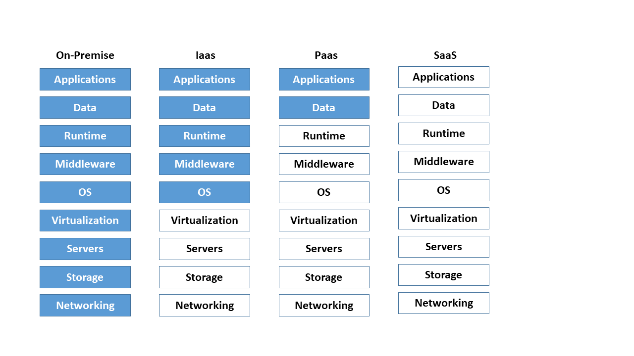
Figure 5: Comparison of the different cloud computing models.
As soon as the term cloud is mentioned, it predominantly refers to a specific usage model of cloud computing. The various types of these usage models are defined below: 21
- Private cloud: The English term "private" translates into German as "privat" and, in the context of cloud, stands for "not for the public". A company uses a private cloud in a secure environment such as its own internal network. This does not necessarily mean that the IT infrastructure used is the property of the company, as it can also be provided by third parties. Private merely clarifies that a company is the sole user of this model. This has the advantage that it retains control in terms of data protection, even if third-party providers such as Amazon or Microsoft manage private cloud environments.
- Public cloud: A public cloud provides access to abstracted IT infrastructures and services for a large number of users. Customers can use services and infrastructures via the Internet. Examples are file hosting services such as Google Drive from Google Inc. or Dropbox from Dropbox Inc.
- Hybrid cloud: A hybrid form of the two variants mentioned above is the hybrid cloud. Users are offered the option of processing business-critical data with a focus on data protection in private cloud environments. Non-sensitive data is made available in the public cloud using cloud services such as IaaS or PaaS on the Internet. Hybrid clouds offer a further advantage in that performance peaks occurring at short notice are compensated for by shifting services from the private to the public cloud. Hybrid clouds enable the gradual merging of public and private cloud services in order to be able to utilize existing infrastructure hardware for as long as possible.
Figure 6 shows an overview of private, public and hybrid cloud environments and illustrates the relationship between a private and public network. For example, a private network is a VPN, while the Internet belongs to the public network segment.
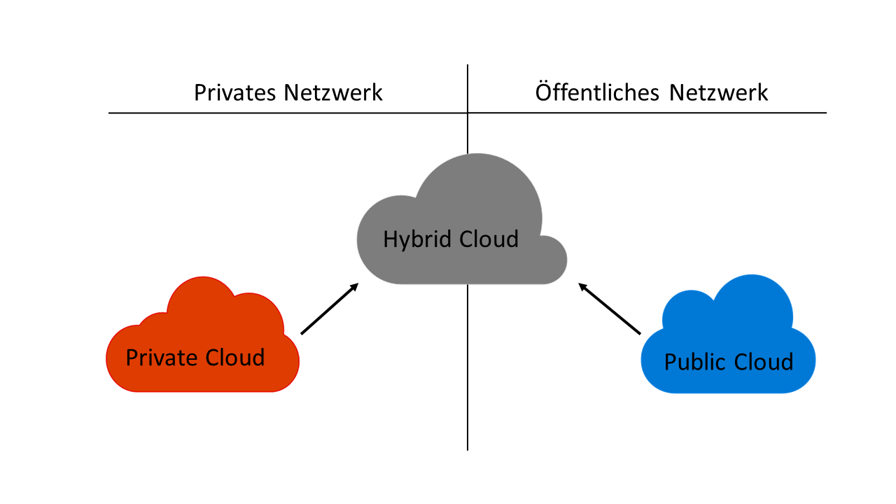
Figure 6: Relationship between public, private and hybrid cloud models.
Other noteworthy business models in which cloud computing is subdivided are community cloud, virtual private cloud and multi-cloud, which we will not discuss in detail in this paper.
Cluster
A cluster is a computer network and usually refers to a group of at least 2-n servers, also called nodes. All nodes are connected to each other via a local area network (LAN) and form a logical unit of a supercomputer. Gregory Pfister defines a cluster as follows: 22
"A cluster is a type of parallel system that consists of interconnected whole computers and is used as a single, unified resource. “ 23
Clusters are the approach to achieving high performance, high reliability, or high throughput by using a collection of interconnected computer systems. Depending on the type of setup, either all nodes are active at the same time to increase computing power, or at least 1-n node is passive so that it can stand in for a failed node in case of failure. For data transmission, all servers are connected to each other via at least two network connections to a network switch. Two network connections are typical, since on the one hand the switch is excluded as SPOF, and on the other hand to be able to realize a higher data transfer. 24
With reference to the current Top 500 list of the world's fastest computers, the term supercomputer is absolutely appropriate. It is clear that several cluster systems are among the ten fastest computers in the world. Computer clusters are used for three different tasks: providing high availability, high performance computing and load balancing. 25
Shared and distributed storage
According to the von Neumann architecture, a computer has a shared memory that contains both computer program instructions and data. Parallel computers are divided into two variants in this respect, systems with shared or distributed memory. Regardless of which variant is used, all processors must always be able to exchange data and instructions with each other. The memory access takes place via a so-called interconnect, a connection network for the transfer of data and commands. The interconnect in clusters is an important component for exchanging and communicating data between management and load distribution processes. 26
In systems with shared memory, all processors share a memory. The memory is divided into fixed memory modules that form a uniform address space that can be accessed by all processors. The von Neumann bottleneck comes into play here, which means that the interconnect, in this case the data and instruction bus, becomes the bottleneck between memory and processor. Due to the sequential or step-by-step processing of program instructions, only as many actions can be performed as the bus is capable of. As soon as the speed of the bus is significantly lower than the speed of the processors, the processors repeatedly have to wait. In practice, the waiting time is circumvented by the use of buffer memories (cache), which is located between the processor and the memory. This ensures that program commands are available to the processor quickly and directly. 27
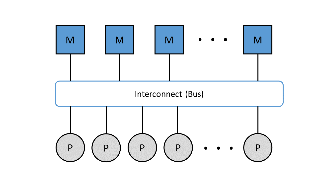
Figure 7: Parallel computers with shared memory connected via the data and instruction bus.
Figure 7 shows the representation of memory (M) and processors (P) connected via the interconnect.
Computer systems with distributed memory, on the other hand, have a separate memory for each processor. In this case, a connection network is required. As soon as a shared memory is dispensed with, the number of processors can be increased without any problems. By using a distributed memory, each processor gains the upper hand over its address space, since it is allocated its own local memory. Similar to distributed memory, communication takes place via an interconnect, which in this case is a local network. The advantage of computer systems with distributed memory is the increase in the number of processors, but the disadvantage lies in the disproportion between computing and communication performance, since the transport of data between CPU (Central Processing Unit) and memory is much slower. The bottleneck is not in the bus as with distributed memory, but in the local network. 28
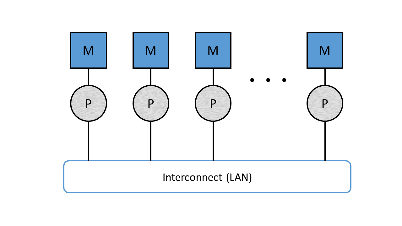
Figure 8: Parallel computers with distributed memory, connected via a local area network.
As soon as processor systems are operated with shared memory, through the use of multi-core processors, the complexity and expense of the electronics to be implemented increases. This consequently entails higher costs. A single system with, for example, 128 multicore processors is very expensive and is therefore out of the question for massively parallel applications. It is far more cost-effective to operate 128 PCs, for example, with the same hardware, each with one processor and distributed memory.
Message Passing Interface
Message Passing Interfaces (MPI) is a standardized and portable message passing standard for message transmission between cluster nodes with distributed memory (see Figure 9). This concept was developed by a group of researchers from academia and industry to enable the development of a variety of parallel computing architectures. The standard defines syntax and semantics that are useful to a wide variety of users. It is not a standardized protocol, but acts as a programming interface for serial code used by the C and Fortran programming languages. MPI is the most widely used model for parallel and concurrent programming today. Currently used MPI implementations are MPI/Pro and Local Area Multiprocessor (LAM) MPI. Both implementations are now fixed components of Linux distributions. Another message-based model is the Parallel Virtual Machine (PVM) platform. This allows several computers with a Windows or Linux operating system to be combined to form a parallel system with distributed memory. 29
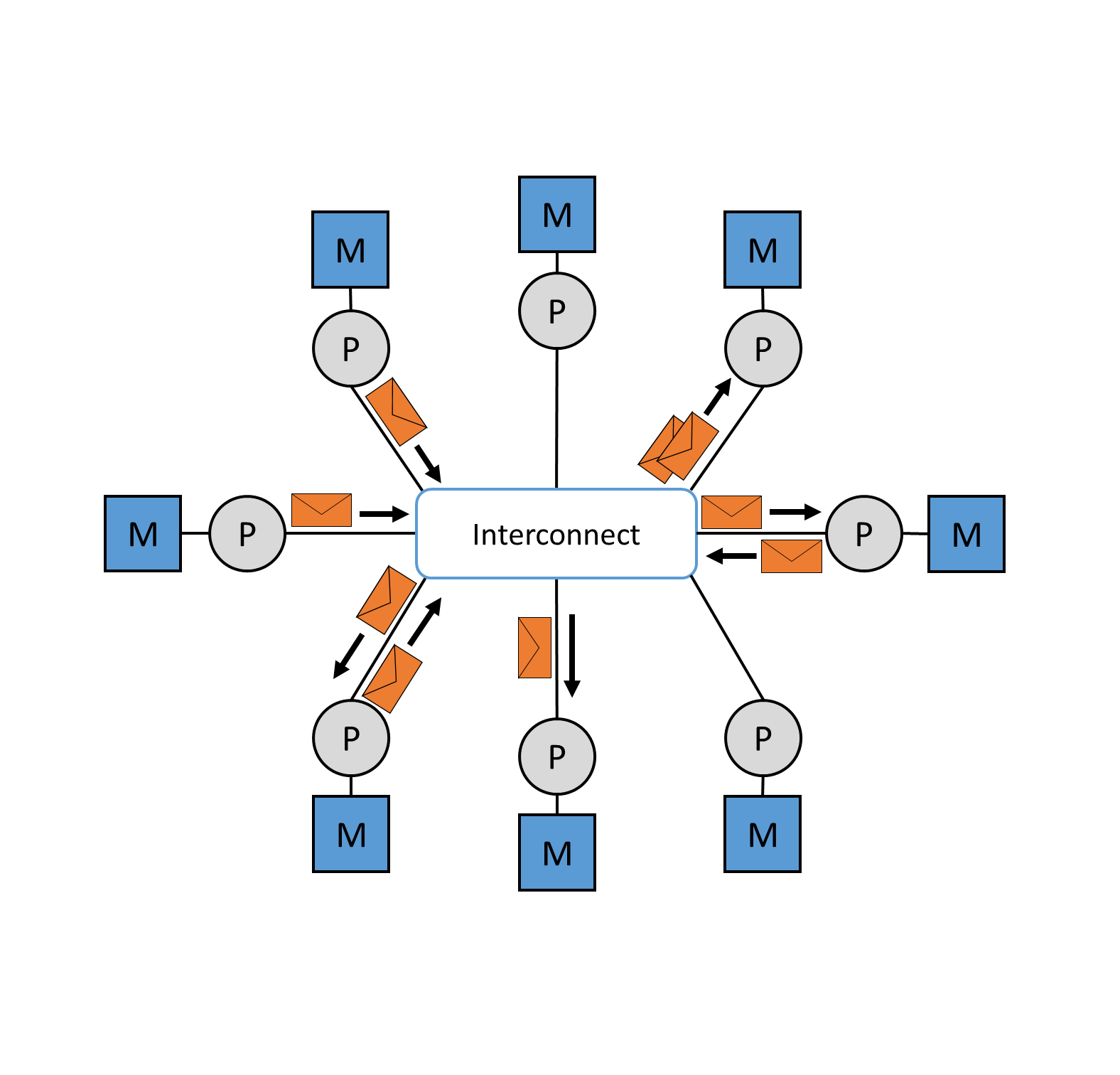
Figure 9: Message transmission between cluster nodes via the interconnect.
High-Availibility Cluster
There are many different application scenarios for clusters. The most popular uses are high-availability (HA), high-performance computing (HPC) and load balancing (LB). These types of computer networks are subdivided as follows in the diagram below.
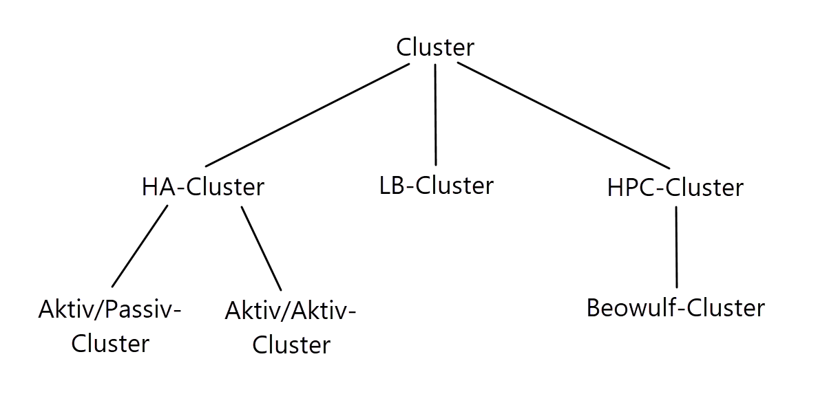
Figure 10: Subordination of the different cluster types.
High availability cluster or failover cluster pursues the goal of avoiding one or more single points of failure. In a cluster, a specific system component is defined as SPOF as soon as it is designed as non-redundant. A failover cluster is a group of servers configured so that if one or more servers fail, another server automatically takes over their service and continues processing. Each server in the cluster has at least one other teammate, which functions as a so-called standby server or partner server. The simplest variant of an HA cluster is usually found in the 2-node solution, which is either symmetrically or asymmetrically structured, depending on the architecture. An asymmetrically structured cluster is an active/passive cluster, i.e. as soon as one of the nodes has a fault, its passive partner node steps in and takes over its services and function. A symmetrical active/active cluster, on the other hand, keeps both server nodes active. In this case, various services are shared between the two nodes for load balancing. In this case, high availability and load balancing are provided at the same time.
If one of the nodes fails, the active partner takes over its services and the cluster remains available, not highly available but still in a running mode. 30
For a standby server to be able to step in as an active server at all, it must use a certain technique to determine that its active partner server is no longer functioning. This is usually done by a so-called heartbeat mechanism. This typically runs as a service on both server nodes. The communication between the services runs over a local, dedicated as well as redundant network. They communicate with each other and check each other for signs of life - their heartbeat. As soon as there are more than 2 nodes in a cluster, they also monitor each other using various heartbeat techniques. Using push heartbeat, active servers send signals to their respective standby servers at a fixed interval. If one of the standby servers no longer receives a signal, it assumes that its partner has failed and takes over the active role. Based on a pull heartbeat, the standby server sends a certain number of requests to its active partner. If the limit of these requests is reached without a valid response from its partner, the partner takes over its services and thus assumes the active part. 31
High-Performance Computing Cluster
The goal of HPC clusters is to process complex computing tasks or simulation applications, in parallel on all cluster nodes. The combination of all cluster nodes thus results in immensely high computing power. All nodes must consist of homogeneous or similar hardware components in order to simplify the administration effort and maintenance and to be able to handle error sources more easily. Furthermore, all nodes are connected to each other via a local network and usually access a common data storage. As soon as an application falls into one of the following categories, increased requirements are placed on memory, network and processors:
- computing-intensive applications
- memory-intensive applications
- communication-intensive applications
Because of this, these types of clusters must provide high resilience, high availability, and high redundancy.
The use of high-performance clusters, takes place in particularly computationally intensive applications, which are often used in the scientific field. 32
Figure 11 shows a typical architecture of an HPC cluster. All compute nodes, also called working nodes, are connected via a local network by means of a switch. In addition, there is a so-called shared storage. This should not be confused with shared memory, which is only used in processor systems (see Shared and distributed Storage). Shared storage is used for the joint and simultaneous access and exchange or intermediate storage of data, such as specially required application data or databases. Master nodes or front-end nodes form the central work platform for users, on which they can log in via a console terminal and interact with the cluster. Computing jobs are initiated and applications installed via this platform. 33
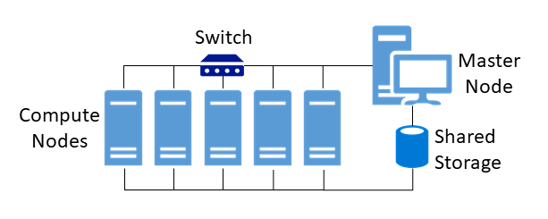
Figure 11: Typical construct of an HPC cluster.
The first multiprocessor clusters trimmed to high-performance computing, such as the VAX-11/780, came onto the market in 1977 under the name VAXCluster or VMSCluster. The technology pioneer at that time was Hewlett-Packard (HP), then under the company name Digital Equipment Corporation (DEC). VAX stands for Virtual Address eXtension and, in conjunction with the OpenVMS(virtual memory system) operating system specially developed for this purpose, was a powerful tool in terms of security, stability and low downtimes. Another notable example of an HPC cluster that focuses more on low-cost high-performance computing is a Beowulf cluster, which we will discuss in more detail in section High-Performance Computing Cluster. 34
Load-Balanced Cluster
Processing large amounts of data can lead to high loads on individual nodes and must be managed. Server nodes have limited CPU, memory or network capacity and cannot handle all loads on their own. Furthermore, certain applications can only use or rely on a certain number of processors. A load-balanced cluster is a computer network optimized for load distribution. By distributing the data volumes over several identical computers, the system is protected against total failures. Likewise, the function of uniform performance availability is maintained as capacity or computational requirements change during operation. Figure 12 shows a cluster-internal load balancer that distributes client requests evenly across all servers. 35
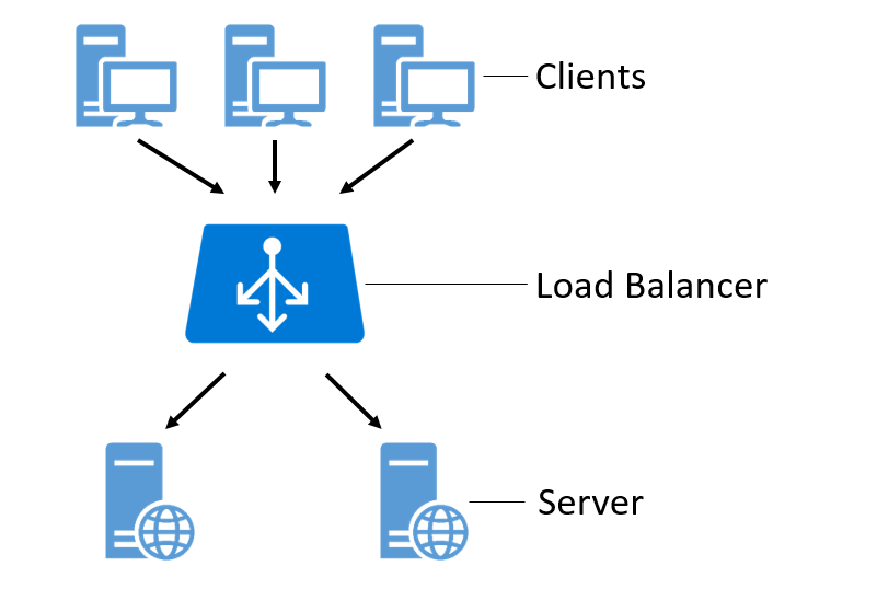
Figure 12: A cluster-internal load balancer distributes client requests evenly to all servers.
Management for intelligent distribution of data streams is handled by these various distribution algorithms:
-
Round-Robin algorithm: All computational requests and loads are distributed evenly to each server, regardless of the current number of connections or response times. Round-robin is best suited when the servers in the cluster have equal processing capabilities based on hardware. Otherwise, some servers will receive more requests than they can handle, while others will consume only a portion of their resources.
-
Weighted Round-Robin: A weighted round-robin algorithm takes into account the different processing capabilities of each server. Users manually assign a performance weight to each server, and a scheduling sequence is automatically generated depending on the server weight. Requests are then routed to the different servers according to a round-robin scheduling sequence. This algorithm makes sense as soon as one or more servers have different performance strengths and maintain a performance equilibrium according to their weightings.
-
Least-Connection Algorithm: Only requests are sent to the server in a cluster based on which currently serves the fewest connections.
-
Load-Based Algorithm: Similar to Least-Connection, only certain requests are sent to the cluster; in a load-balanced algorithm, only requests are sent to servers that currently have the lowest load.
Beowulf Cluster
A Beowulf Cluster is a computer design that provides parallel processing across multiple computers to create a low-cost, high-performance supercomputer. The name Beowulf, translated into German, means werewolf and, in this context, comes from an Old English heroic poem and has since stood as a meaningful emblem of the power such a cluster can deliver. The first clusters of this type were developed in 1994 by scientists Thomas Sterling, Donald Becker and Phil Merkey to support the Earth and Space Sciences Project (ESS) at the National Aeronautics and Space Administration (NASA). 36
A Beowulf Cluster in practice is typically a collection of generic computers, either commodity PCs or larger server systems, that are independently procured, assembled, and connected via an internal network. A Beowulf cluster consists of two types of computers, a main (master) computer and multiple computer nodes. When a complex problem or large data set is given to a Beowulf cluster, the master computer first runs a program that breaks the problem into small pieces and sends one piece at a time to each node to compute. When the nodes finish their tasks, the master continuously sends more pieces to them until the entire problem is solved. 37
When Thomas Sterling and Donald J. Becker started up their cluster in 1994, it consisted of sixteen Linux PCs, each with 100 MHz Intel DX4 processors. The individual computers were connected via Ethernet for the required data exchange. Several benchmark tests were performed, which test the performance of computers by measuring the number of floating point number calculations possible per second. The measurement is given in Floating Point Operations Per Second (FLOPS). The results of the tests were surprising with 4.5 MegaFLOPS per node and 60 MegaFLOPS in total. This corresponds to a speedup of 13.33 or an efficiency of 83%. These results are impressive for the reason that this performance was comparable to the supercomputers from IBM and Co. at the time. The remarkable thing, however, is that this cluster was operated at only a fraction of the cost of supercomputers. 38
The following figure shows a Beowulf cluster with 64 PC nodes, which was developed by Phil Merkey at Michigan Technological University, also for the ESS project.
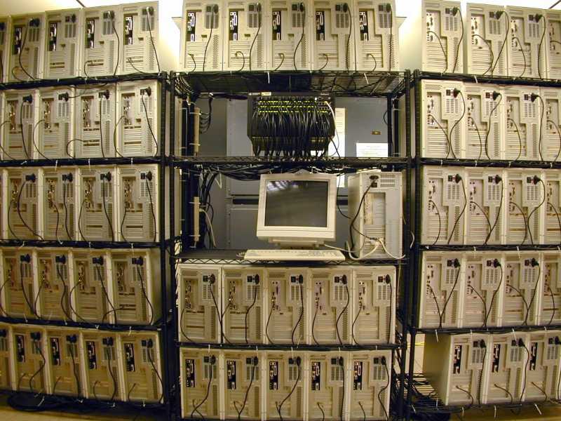
Figure 13: A 64-node Beowulf cluster from Michigan Technological University.
Virtualization
Before we delve a little deeper into the chapter Container Management Systems (see Container Management Systems), we will look at the basic technology of virtualization. This foundational technology is necessary for the operation of container technologies like Docker. In computer science, virtualization refers to the creation of a virtual, rather than actual, version of something, such as an operating system, server, storage device, or network resources. Virtualization refers to a technology in which an application or an entire operating system is abstracted from the actual underlying hardware. In connection with container technologies, a well-known type of virtualization, we distinguish here between two techniques of virtualization, hypervisor-based and container-based virtualization. 39
Hypervisor-based virtualization
A key application of virtualization technology is server virtualization, which uses a software layer called a hypervisor to emulate hardware such as memory, CPU, and networking. The guest OS, which normally interacts with real hardware, implements this with a software emulation of that hardware, and often the guest OS has no idea it is running on virtualized hardware. The hypervisor decides which guest OS gets how much memory, processor time and other resources from the host machine. In this case, the host machine runs the host OS and the hypervisor. This means each OS appears to have direct access to the processor and memory, but the hypervisor actually controls the host processor and resources by allocating what is needed by each OS. While the performance of this virtual machine does not match the performance of the OS running on real hardware, the concept of hypervisor-based virtualization works quite well because most OSes and applications do not require full use of the underlying hardware. This allows for greater flexibility, control and isolation by eliminating dependency on a specific hardware platform. Originally intended for server virtualization, the concept of virtualization has expanded to applications, which is implemented using isolated containers. 40
Container-based virtualization
Container virtualization or container-based virtualization is a method of virtualizing applications but also entire operating systems. Containers in this sense are isolated partitions that are integrated into the kernel of a host machine. In these isolated partitions, multiple instances of applications can run without the need for an OS. This means that the OS is virtualized, while the containers that run inside the system have processes that have their own identity and are thus isolated from another process in another container. Software running in containers communicates directly with the host kernel and must be executable on the operating system and CPU architecture on which the host is running. By not emulating hardware and booting a complete operating system, containers can be started in a few milliseconds and are more efficient than traditional virtual machines. Container images are typically smaller than virtual machine images because container images do not need to contain device drivers or a core to run an operating system. Because of the compactness of these application containers, they find their predominant use in software development. Developers do not have to set up their development machines by hand; instead, they use pre-built container images. These images are memory maps of entire application structures that can be arbitrarily moved back and forth between different host machines, also called shipping. This is one of the reasons why container-based virtualization has become increasingly popular in recent years. 41
Examples of container platforms are Docker from Docker Inc. and rkt from the developers of the CoreOS operating system, with Docker enjoying increasing popularity in recent years. Compared to virtual machines, Docker represents a simplified solution to virtualization. 42
Figure 14 shows the key difference between container-based and hypervisor-based virtualization.
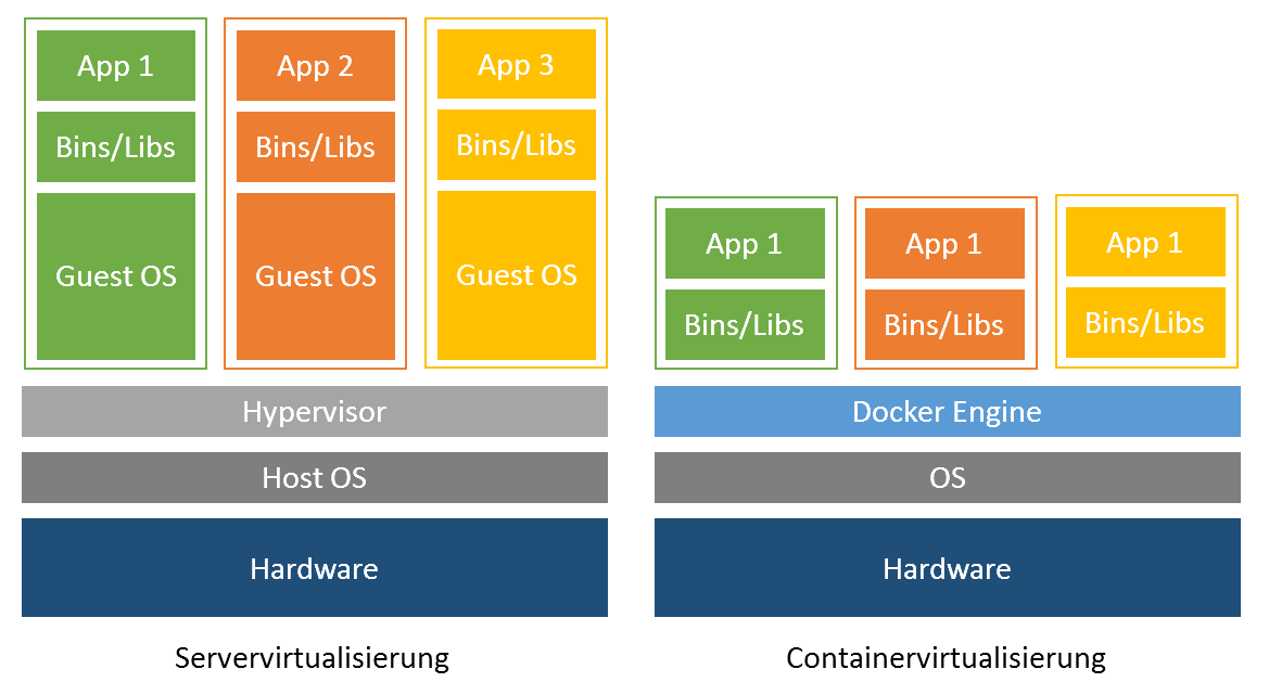
Figure 14: Comparison between hypervisor and container.
Container Management Systems
As soon as several containers are to be distributed and run on a parallel system such as a cluster, it is necessary to use a container management system. Such a system manages, scales and automates the deployment of application containers. Well-known open source systems are Kubernetes from Google or Docker Swarm. Another very well-known container manager worth mentioning is the OpenShift software from Redhat, but we will not discuss it further in this paper. These cluster management tools play an important role as soon as a cluster has to take care of tasks such as load balancing and scaling. In the following, we will introduce the first two container managers mentioned and explain their structure and use with containers.
Docker Swarm
Docker is an open standards platform for developing, packaging, and running portable distributed applications. With Docker, developers and system administrators can create, deliver, and run applications on any platform, such as a PC, the cloud, or a virtual machine. Obtaining all the necessary dependencies for a software application, including code, runtime libraries, and system tools and libraries, is often a challenge when developing and running an application.
Docker simplifies application development and execution by consolidating all the required software for an application, including dependencies, into a single software unit called a Docker image that can run on any platform and environment. The Docker software, based on the Docker image runs in an isolated environment called a Docker container, which contains its own file system and environment variables. Docker containers are isolated from each other and from the underlying operating system. 43
One solution already integrated into Docker is Docker Swarm Mode. Docker Swarm is a cluster manager for Docker containers. Swarm allows administrators and developers to set up and manage a cluster consisting of multiple Docker nodes as a single virtual system. Swarm mode is based on Docker Engine, the layer between the operating system and container images. Clustering is an important feature for container technology because it creates a cooperative group of systems that provides redundancy and enables failover when one or more nodes experience a failure. A Docker Swarm Cluster provides users and developers the ability to add or remove containers as compute requirements change. A user or administrator controls a swarm through a swarm manager, which orchestrates and deploys containers. Figure 15 shows the schematic structure and relationship between instances. 44
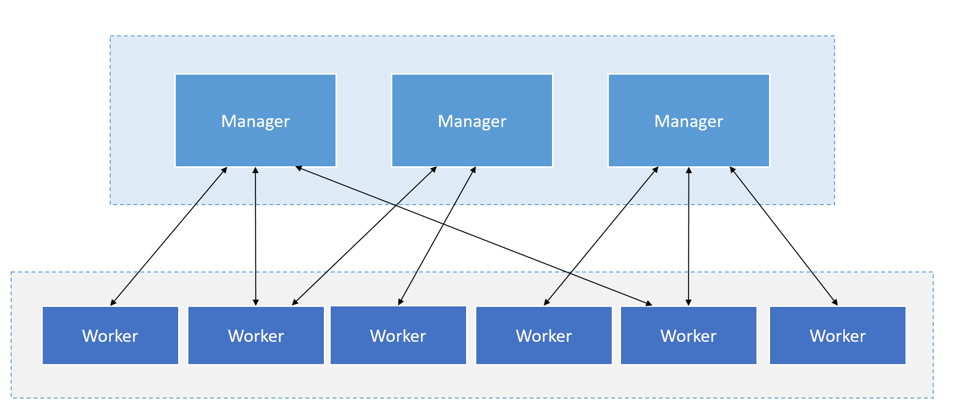
Figure 15: Structure and communication of the manager and worker instances.
The Swarm Manager allows a user to create a primary manager instance and multiple replica instances in case the primary instance fails, similar to an active/passive cluster. In Docker Engine's swarm mode, the user can provision so-called master nodes and worker nodes at runtime. 45
Google Kubernetes
The name Kubernetes comes from the Greek and means helmsman or pilot. Kubernetes is known in specialist circles by the acronym K8s. K8s is an acronym where the eight letters "ubernete" are replaced by "8". Kubernetes provides a platform for scaling, automatically deploying and managing container applications on distributed machines. It is an orchestration tool and supports container tools such as Apache Mesos, Packer, and including Docker. 46
A Kubernetes system consists of master and worker nodes, the same system principle as Docker Engine, with manager instances named master. The smallest unit in a Kubernetes cluster is a pod and runs in the worker nodes. This pod consists of at least one or more containers. A worker node can in turn run multiple pods. A pod is a worker process that shares virtual resources such as network and volume among its containers. 47
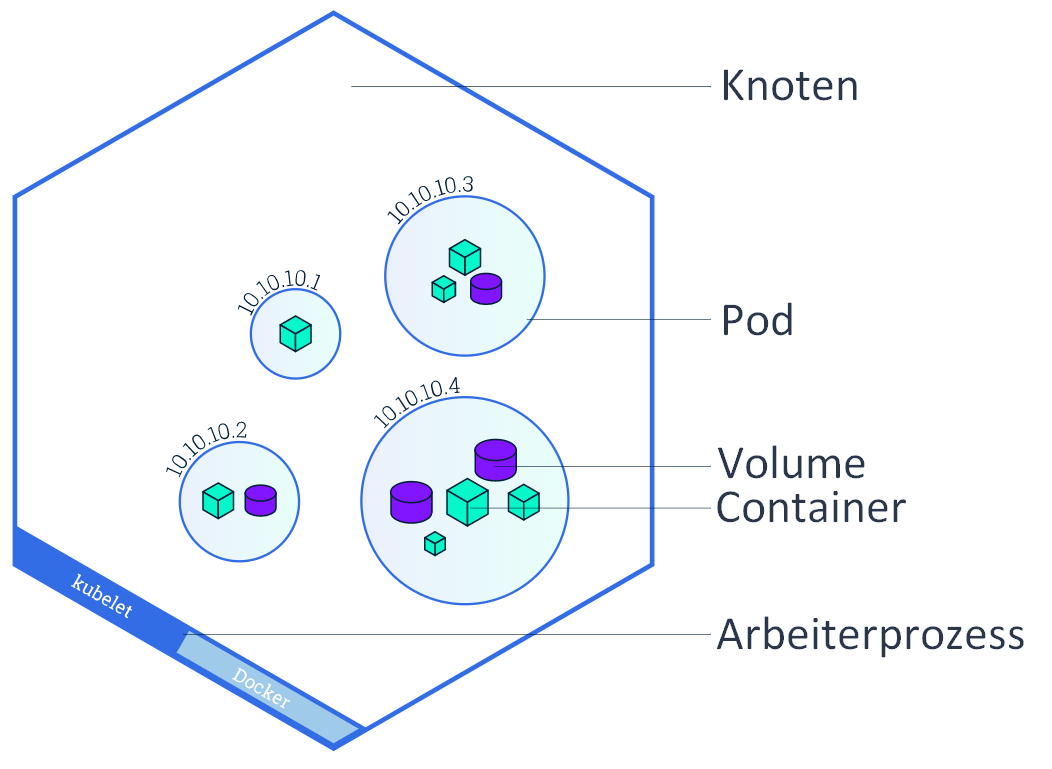
Figure 16: Granular representation of node, pod and container.
The following services run on the individual worker nodes: 48
- Docker: providing the container engine.
- kubelet: Agent, which takes over the management of the containers.
- kube-proxy: Service that handles network management and port forwarding to and from containers.
The main nodes take care of the management and controlling of all nodes. The following services are divided here: 49
- kube-apiserver: User interface to the nodes.
- etcd: Storage location of the cluster configurations, the so-called key-value store.
- kube-scheduler: The scheduler determines, depending on the available resources, which worker nodes are assigned which pods.
- kube-controller-manager: This manager service takes over the controlling functions and monitors if all nodes are working, which pods are assigned to which service and manages port forwarding.
Raspberry Pi
Credit-card-sized single-board computers (SBCs) such as the Raspberry Pi, developed in the UK by the Raspberry Pi Foundation, were originally intended to promote computer science education in schools. Acronyms like "RPi" or the abbreviation "RasPi" or "Pi" for the Raspberry Pi are mostly common here. Like smartphones, single-board computers are equipped with ARM processors (Advanced RISC Machines). Before the development of ARM in 1983, there were mainly CISC and RISC processors on the market. CISC stands for Complex Instruction Set Computer. Processors with this architecture are characterized by extremely complex instruction sets. Processors with RISC (Reduced Instruction Set Computer) architectures, on the other hand, have a restricted instruction set and therefore also operate with low power requirements. The Pi's board is equipped with a system-on-a-chip (SoC, i.e. single-chip system), which has the identifier BCM2837 from Broadcom. The SoC consists of a 1.2 GHz ARM Cortex-A53 Quad Core CPU, a VideoCore IV GPU (Graphics Processing Unit) and 512 MB of RAM. It does not include a built-in hard drive, but uses an SD card for booting and permanent data storage. It has an Ethernet port based on the RJ45 standard for connecting to a network, an HDMI port for connecting to a monitor or TV, USB (Universal Serial Bus) ports for connecting a keyboard and mouse, and a 3.5 mm jack for audio and video output. 50
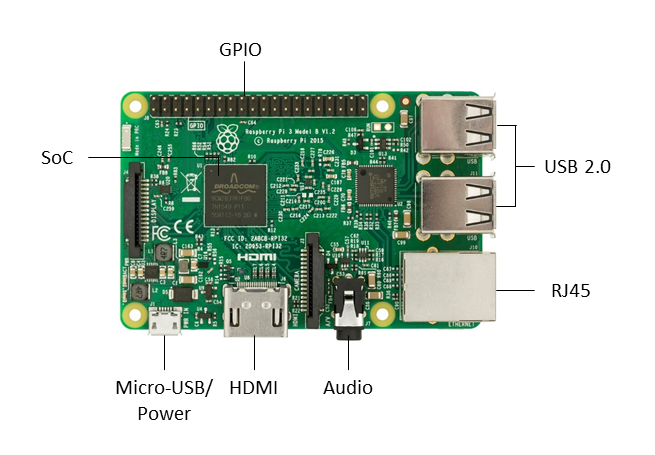
Figure 17: Illustration of a Raspberry Pi 3 Model B and its components.
An average of 35 EUR is the price one pays for a Raspberry Pi, which makes it economically suitable for use and integration into a cluster system, since the unit costs for individual nodes are low. 51
General Purpose Input Output (GPIO) is the name for programmable inputs and outputs for general purposes. A Raspberry Pi has a total of 40 GPIO pins, twelve of which are for power supply and 28 of which serve as an interface to other systems in order to communicate with or control them. GPIO pins 3 and 5 (see Figure 18) enable devices such as an LCD display to be addressed by means of an Inter-Integrated Circuit (I2C), a serial data bus.
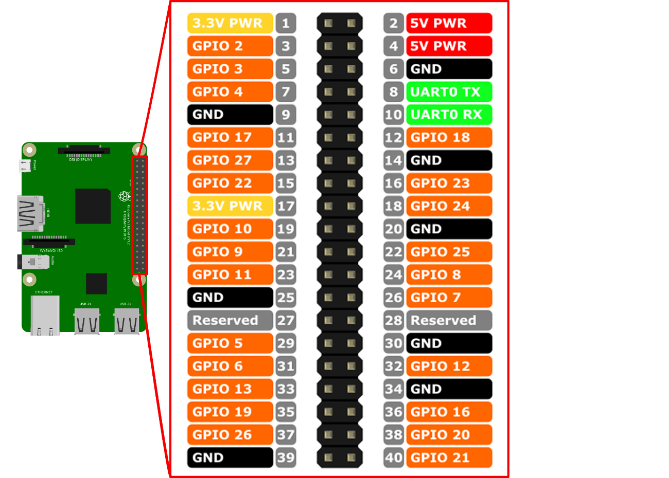
Figure 18: Illustration of the different GPIO pins of the Raspberry Pi.
Conception and design
In this chapter, we will go into the basic concept of creating a cluster using Raspberry Pi single-board computers. Here, these mini-computers form the basis for constructing a cost-effective and energy-efficient cluster system. Inspired by Joshua Kiepert and his 32-node RPiCluster or Nick Smith and his first design of a 5-node Raspberry Pi cluster, the idea of further developing and improving certain components has emerged, such as increasing the cooling performance by means of an optimized airflow supply, adding and logically arranging further connection possibilities and considering a modular expandability of the cluster. 52
Requirements
The main focus in the design of this Raspberry Pi cluster is on the following requirement criteria:
- Cost Efficiency.
- Energy efficiency.
- Scalability.
- Resilience.
Further criteria are a visual and easy-to-read status and information display of current system values, ideal cooling and optimization of the airflow for the best possible removal of heat. Furthermore, the entire design concept is fundamentally based on certain design requirements, which we will discuss in more detail in the design decisions (see Design decisions).
Cost and energy efficiency
The factors of cost and energy efficiency are paramount and predominantly influence the conception and design. In order to keep the acquisition costs as low as possible but still be able to offer efficient computing power, Raspberry Pi single-board computers in version 3 are to be installed. The use of unnecessary cable lengths or heavy and expensive materials such as sheet steel or aluminum for the housing should be avoided. In addition, a weight and further cost saving is to be achieved by using plastic instead of steel screws.
The system should be reproducible at low cost and consume as little power as possible. Energy consumption of less than 60 kilowatts per hour is planned, which is comparatively equivalent to the average power consumption of a commercially available light source such as an incandescent lamp. Such low power consumption implies the portability factor, which means that it should also be possible to use this cluster on a mobile basis.
Scaling and resilience
Scaling is to be considered in this system in two respects. On the one hand, the user should be given the option of connecting the entire system with other clusters in order to be able to scale cluster-wise at this level. Here we also speak of horizontal scaling. On the other hand, it should be possible to scale vertically or node by node within a cluster by adding or removing individual nodes. This is done either automatically using cluster software or by physically adding or removing further single-board computers. Due to the modular structure of the cluster, the primary goal is to expand individual entire clusters, i.e. vertical scaling.
In parallel to scaling, failover is an important player when it comes to keeping the cluster alive. As soon as the cluster system scales on the software side, all peripheral components must be designed and optimized accordingly so as not to reach their physical limits, such as maximum storage capacity or computing power. This also applies to components such as the network distributor and the power supply unit. With the help of organizational measures and the creation of technical redundancies, this fail-safety is to be guaranteed. This is also referred to as system availability.
Status and information display
For a direct perception of current system values such as host name, system time, processor and case temperature, a visual information display should be available in the form of a display. These important and system-critical values should be immediately and directly readable without the help of technical means, such as a keyboard or the connection of an external monitor. Furthermore, this display should have a backlight to be readable even in dark rooms or with little to no light.
Cooling
Passive cooling and optimized case ventilation are important points that have to be considered in the design. The advantage of passive cooling should be used to save energy on the one hand and costs on the other. Active cooling is nevertheless necessary to ensure the supply of cold air and the removal of warm air. Likewise, a basic law of physics, the so-called chimney effect, must not be lost sight of during further planning. This states: warm air rises, cold air remains on the ground.
Air flow and heat dissipation
The processors of the individual nodes and integrated circuit modules (IC) or internal circuit modules of the individual peripheral components develop a certain amount of heat during operation. For a correspondingly good removal of this warm air and to avoid heat accumulation inside the case, this should be done in several stages and can only be ensured with the help of an active case fan:
-
Absorption of cold outside air at the front and transport to the passive cooling elements inside the housing.
-
Dissipation of heat from the surface of the components (CPU, IC)
-
Removal of heated air from the rear of the housing.
The design of the case should be adapted accordingly so that the supplied air flow can optimally flow into the case, include all components in its air channel as far as possible and discharge warm air from the passive cooling elements out of the case again at a suitable point.
Connections
Due to the compact design of the housing, planning and accommodating all necessary connections poses a certain challenge. It is important to avoid unnecessary cable lengths within the housing, to save space and to ensure sufficient room for suitable air circulation. Connections should therefore be located in the immediate vicinity of the components, as should the connections of internal components such as power, network or control cables. In addition, the following connections should be available externally on the housing:
- 1x current
- 2x network
- 1x HDMI
- 2x USB
Modularity
The building block principle, also called modularity, is related to future extensions or the connection of further cluster systems on a modular basis. This means that it should be possible to combine several cluster systems of the same type to form a larger cluster complex. The prerequisite for this are interfaces. In this case, a second network connection (see Connections). Modularity is also a prerequisite for the planned scalability of the overall system and is therefore considered an important point.
Design decisions
The basic characteristics of this Raspberry Pi cluster are minimalism, transparency and simplicity. Minimalism in architecture, be it in building or model construction, is characterized by the reduction to simple cubic forms. The goal is the formation of geometric and pure forms, which is made possible with the help of transparent building materials such as glass. Whereupon we come to the property transparency. On the software side, transparency means that the user of this system knows exactly how the cluster system works, how it scales or what software is used. On the hardware side, it is clear which physical components such as cables, network distributors or connectors are connected to each other or whether systems emit visual signals. Simplicity, on the other hand, stands for easy understanding of the system. It should, at first glance, imply the usefulness of this system, from the point of view of an ignorant as well as affine user.
Minimalism and transparency: cube
We decide on a compact and portable design in the form of a cube and christen the system with the name PiCube. The Pi, as in Rasperry Pi, stands for Python Interpreter and signals that this system supports the Python programming language or is generally supported by all common operating systems like Raspbian or CoreOS. Python convinces with its minimalistic and easily understandable programming style and also contributes to the overall concept of this system. The English word Cube means cube. Another idea for the naming is PiKube, where Kube stands for the cluster management system used and at the same time comes from Kubus, the ancient Greek kybos or the Latin cubus for cube. However, since the design of the cube case does not have exactly equal faces, we decide to use PiCube, since a cube is a regular hexahedron. A hexahedron has six faces of equal size.
Simplicity: Elastic Clip Concept
In order to allow easy assembly and reassembly, without the use of additional tools or fastening screws of any kind, the Elastic Clip concept by Patrick Fenner was used. This concept allows to create a slim and elegant design. For this purpose, we use acrylic glass, which is transparent, light and flexible, as the construction material for the housing. The clips give the possibility to connect the single acrylic glass sides of the cube in a 90 degree angle. The real highlight here is the automatic snap-in of the clip connections in the insertion openings provided for this purpose. Removal or dismantling of the cube walls is done by bending the clip, so that the connections can be released. 53
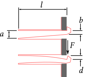
Figure 19: Illustration of clip dimensions with and without force application.
$F$ stands for the force applied to the clip. The clip dimensions are:
$a$ = 4mm, $b$ = 2m, $d$ = 2mm, $l$ = 25mm
Depending on the nature, flexibility and material of the acrylic glass used, the clip may break if too much force is applied. The problem is that the maximum force is applied to the upper right $F$ on the upper right end of the clip, which will break if it is too short. $l$ the clip breaks if it is bent too much or subjected to too much load. To counteract this, there is a simple way to distribute the load on the clip at maximum force by widening the cut. This reduces the risk of the clip breaking. 54
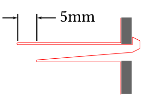
Figure 20: Widening the incision site increases durability.
Due to the material nature and flexibility of acrylic glass, the use of this elastic clip concept is most suitable. If other materials such as medium-density fiberboard (MDF) or simple wood are considered, it must be noted here that due to the unidirectional or one-sided wood fibers, much weaker resistance and thus less flexibility is offered to bend the clip elastically. Use in conjunction with MDF is an alternative, but the clip will inevitably break under too much load.
PiCube
2D model and logo
Inkscape is a professional software for editing two-dimensional (2D) vector graphics. With the help of this software we create a 2D graphic of the housing plates. Prior to manufacturing the enclosure, we sketch and produce a two-dimensional template to determine the exact dimensions for connections, fasteners, and required air slots. Likewise, we are able to determine the exact cutting dimensions and positioning for the elastic clips (see Design decisions) to the millimeter. 55
In the following figure, all six sides are shown and marked accordingly. L for left side, R for right side, F for front, T for top, G for bottom, and B for back. The back contains the connectors for HDMI, network and power, as well as the ventilation grilles and mounting holes for the case fan.
The front has inlets for the double USB socket and the LCD display. Ventilation grilles are also broadly sketched here. All other sides, except the top, also have mounting holes for the rest of the components like the switch, USB charger and the additional side air intakes.
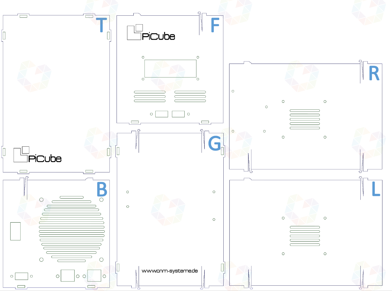
Figure 21: 2D model design of the housing including all connections.
3D model and connections
To ensure that all the required connections (see Connections) can be correctly attached to the housing, we use the Rhinoceros 3D program to create three-dimensional graphics. A 3D model helps to better visualize and represent the housing to be constructed. Physical components can be inserted, rotated or scaled in size. Due to the exact specification of the dimensions of the individual components, a correspondingly realistic model is created before it is manufactured. The rendered graphics (see Figures 22 and 23) show the overall design with all the individual components installed, marked in different colors for better representation. Blue marks the USB components and light gray the case fan. The color dark gray represents network components and red the HDMI port.
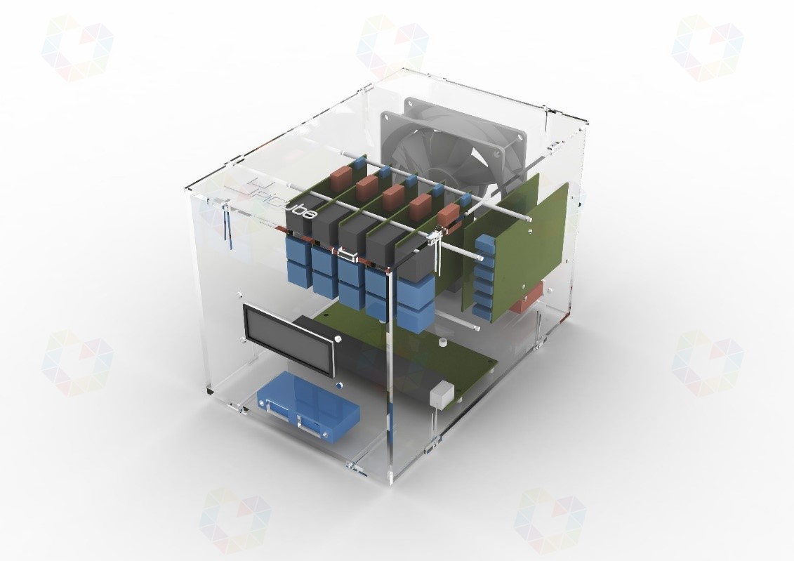
Figure 22: 3D model design including components with a view of the front of the housing.
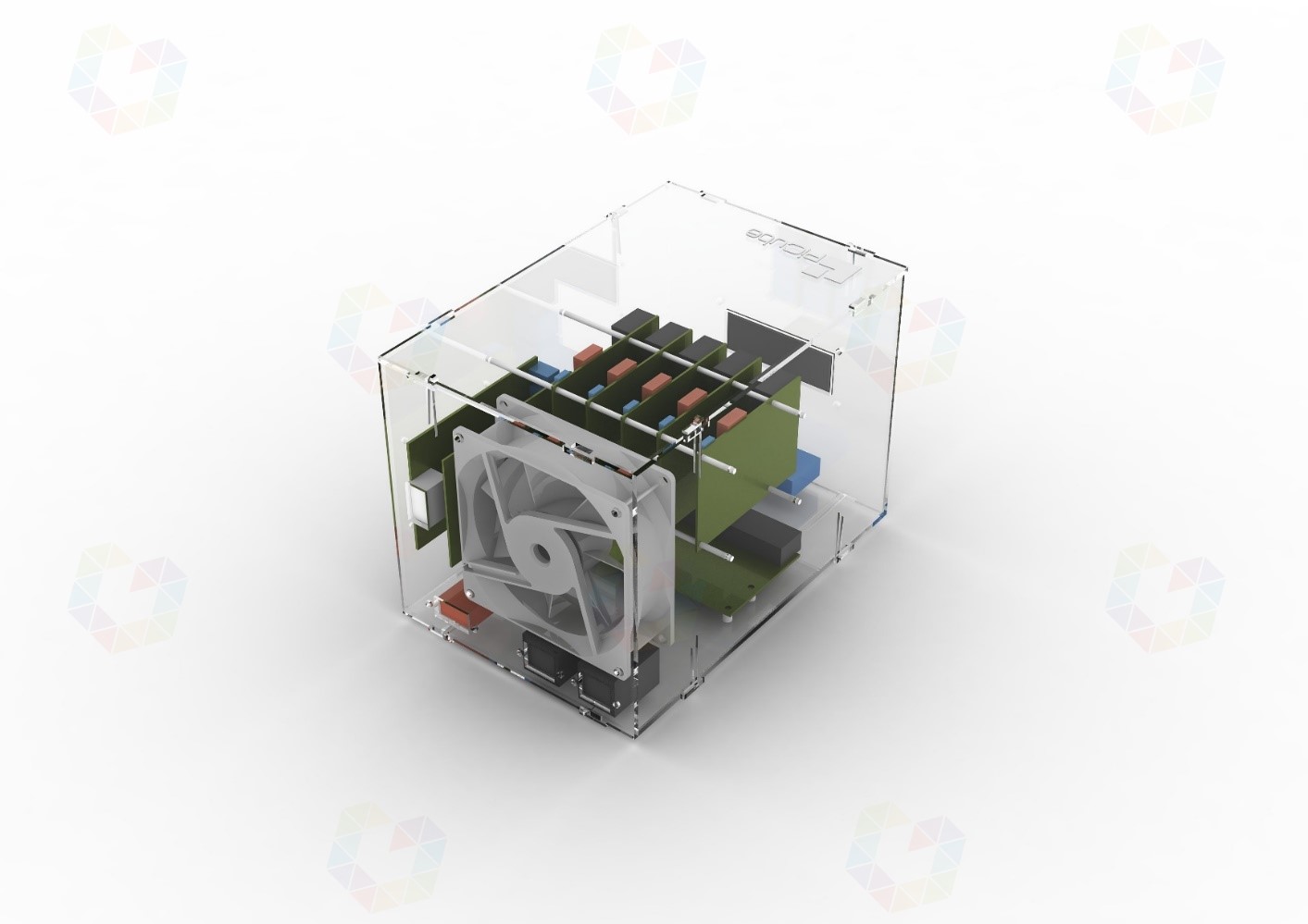
Figure 23: *3D model design including components with view of the back of the housing.*y
Components and costs
For the construction of this prototype, the individual components are obtained from various suppliers or mail-order companies such as Amazon and eBay. The acrylic glass plates are milled in collaboration with Andreas Gregori from MAD Modelle Architektur Design. For the production of the case we do not use laser cutting, but normal milling. This has the advantage that we avoid traces of smoke or sclerosis, which occur during laser cutting due to high temperatures. Milling has another advantage and that is the possibility of surface milling. Thus, we are able to engrave the PiCube logo (see Figures 21 and 24) into the upper and front cube surface.
The five Raspberry Pis and the matching 8 GB SD cards make up the largest part of the costs, amounting to 246.75 EUR. The middle part of the costs, which ranges between 13.75 and 22.99 EUR, is taken up by the Gigabit switch, the USB charger and the USB cables. The rest of the hardware, such as the LCD display, cables and plastic screws, are in the price range of 0.65 to 9.80 EUR.
| Unit(s) | Component | Unit price |
|---|---|---|
| 5 | Raspberry Pi 3 Model B | 42.70 Euro |
| 5 | SanDisk Ultra 8 GB microSDHCUHS -I Class 10 | 6.65 Euro |
| 1 | Edimax ES-5800G V2 Gigabit Switch (8-Port) | 22.99 Euro |
| 1 | Anear 60 Watt USB Charger (6-Port) | 18.99 Euro |
| 5 | Micro USB cable (15 cm) | 2.75 Euro |
| 5 | Transparent power cord (15 cm) | 0.79 Euro |
| 2 | RJ45 jack (female-male) | 2.74 Euro |
| 1 | Dual USB 2.0-A female-male connector | 4.53 Euro |
| 1 | LCD display module 1602 HD44780 with TWI controller | 4.45 Euro |
| 1 | AC 250V 2.5A IEC320 C7 socket | 1.39 Euro |
| 1 | C7 power cable 90 degree angled (1 meter) | 3.26 Euro |
| 1 | Cable jumpers (female-female. 40 wires. 20 cm) | 0.65 Euro |
| 56 | M3 Nylon Hex Spacer Nuts and Bolts White | 0.05 Euro |
| 1 | Antec TRICOOL 92mm 4-pin case fan | 9.80 Euro |
| 1 | Milling cut of the acrylic sheets | 20 Euro |
| Total price incl. VAT | 358.79 Euro |
Table 1: Listing of individual and total price of all components.
Enclosed is a list of all purchased components with price status as of November 30, 2017 (see Table 1). According to the list, the price of all required components for the cluster amounts to a total of 358.79 EUR.
Construction
The practical part of the work, the construction, follows the step-by-step explanation of how to assemble, install and configure the Raspberry Pi cluster. The installation instructions and scripts used in the following are either available from the sources mentioned or from the GitHub repository http://github.com/segraef/PiCube. All installation and configuration steps are easy to follow, so that it is easy to build the cluster on your own.
Mounting and wiring
Elastic clips (see Simplicity) allow the individual case sides to be easily plugged together without the use of screws. The pre-milled holes for the switch, USB charger and LCD display allow the individual components to be attached using the plastic nuts and screws. Pre-milled holes for the LCD display, network ports, HDMI port, and power connector provide the proper slots for the cables to be subsequently connected outside of the case. The assembly is done according to the steps mentioned below:
- Connecting the single board computers together using hex spacers.
- Screw on the attached Raspberry Pis on the left inner side.
- Attachment of the switch to the base plate.
- Attaching the LCD display and USB sockets to the front panel.
- Screwing the USB charger to the right side plate.
- Mounting the case fan, HDMI and network jacks.
After the entire interior has been assembled, the side panels are clipped in step by step. To do this, start with the base plate, onto which the left and right side plates are clipped and clipped together. Before assembling the front panel, we wire the individual components. LCD displays only work by being powered and controlled. A total of 4 cable jumpers are used for this purpose. Two of them are for power and the other two are for control and transmission signals which we connect to GPIO pins 2, 3, 5 and 6 of one of the Raspberry Pis which acts as a master node. All mini computers are connected to the switch using RJ45 network cables. Likewise, we connect the cables of the network jacks to the switch, which serve as network port extensions. Micro-USB cables are typically used for data transfer, in this scenario they are only used for powering the individual single-board computers.
We connect the network switch and all Raspberry Pis to the USB charger using the USB cables. We connect the case fan with its 3-pin connector to the GPIO ports 2 and 6 of one of the Raspberry Pis to supply it with power. After all the necessary cables and components are connected, we move on to the cluster installation. The following two images show the PiCube in a partially and fully wired state.
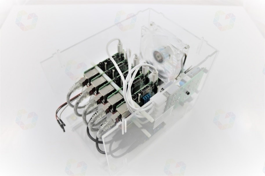
Figure 24: Partially wired PiCube without front and bottom panels.
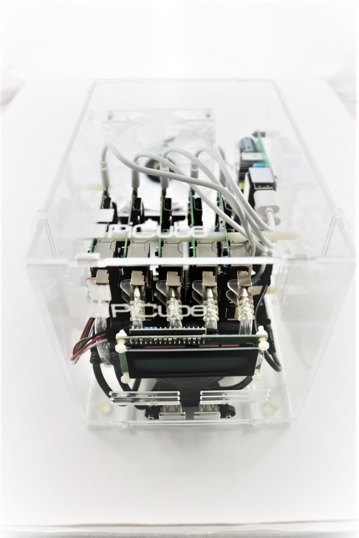
Figure 25: Fully wired and closed PiCube.
Installation
Operating system
To provide a suitable developer system and, to meet all requirements, we use the HypriotOS operating system as the base system for the cluster. The OS provides a Docker-optimized Linux kernel and is therefore ideally suited for this cluster. It already includes all the required modules such as Docker Engine, Docker Machine and Docker Compose. HypriotOS is an operating system specially developed for Raspbery Pi, which is based on the Linux distribution Debian. Important prerequisites for the successful operation of a cluster system are identical and redundantly designed hardware (see Cluster) and the cluster software that can run on it. Among other things, this concerns the same software and driver versions for all participating nodes. To ensure that the cluster system maintains a homogeneous operating system and version structure on all nodes, we use operating system images. 56
Imaging and provisioning
For the installation of Raspberry Pi operating systems, memory images are used. Images are disk images in a compressed file that contains files, file system structures, and boot sectors. Simply put, an image contains an exact disk copy of an operating system. The advantage of using images is that an operating system does not have to be installed. In order for this exact disk copy to be deployed in our nodes, we copy the contents to SD cards and deploy them in our cluster nodes. Using the Hypriot flash tool, the hostname is passed to the image and is thus hardcoded for the first boot of the Raspberry Pi. Hardcoded means that values, such as the hostname in this case, are passed into the startup configuration of the operating system and are called and used when the system starts. The following code snippet (see Listing 1) shows the command that sets the hostname rpi1 for the image package hypriotos-rpi1-v1.6.0.img.zip after downloading the HypriotOS image from the address https://github.com/hypriot/image-builder-rpi/releases/download/v1.6.0/. 57
|
|
Listing 1: The HypriotOS image is downloaded and copied to the SD card using flash.
YAML Ain't Markup Language (YAML) is a markup language and gives us the possibility to create customized parameters for a startup configuration. Thus, it is very easy to pass values into a configuration which will be initialized and applied when each node is started for the first time. Examples for start parameters, which can be preconfigured:
- Hostname
- WLAN -SSID
- WLAN password
- Static or dynamic IPaddress
The YAML files for our nodes look like this, with the hostname for the respective Raspberry Pi adjusted accordingly:
|
|
Listing 2: Example of a YAML configuration.
Fixed WLAN parameters lets individual nodes connect to an existing
wireless network. We copy this configuration to the image in the /boot/
directory. The following code snippet shows setting the YAML
configuration using flash. This accesses /boot/device-init.yaml on
initial startup and copies the appropriate parameters to the operating
system's startup configuration:
|
|
Listing 3: The HypriotOS image is downloaded, copied to the SD card using flash and a given YAML configuration.
Time is precious and, in order to save it, we prepare the respective image for each individual Raspberry Pi and thus take advantage of the automatic provisioning. Due to the use of a total of 5 cluster nodes, the manual installation, configuration and maintenance of each individual node would be very time-consuming. Therefore, we provision every single operating system in advance, which means we use a master image that already contains current driver versions and software packages. We modify this system image for each individual node by means of a YAML configuration, so that only the host name has to be entered and is thus hard-coded or hard-configured. As soon as the system starts, it takes the hardcoded hostname value from its startup configuration and boots with it. Flash is used to provision the remaining 4 nodes with the host names rpi2, rpi3, rpi4 and rpi5 respectively.
Commissioning of the cluster
After all SD cards are prefabricated and inserted into the individual Raspberry Pis, the cluster is put into operation and the system is connected to the power. After all systems get power, the LCD display and the individual LED s of the Raspberry Pis light up one after the other, signaling their operation (see Figure 26). The startup process of the single-board computers happens quite quickly and the systems are ready for the next step, the actual configuration of the cluster, after about 30 seconds.
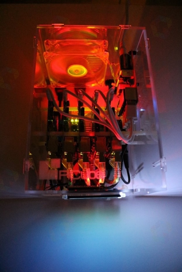
Figure 26: All systems signal their readiness for operation.
Cluster configuration
Installing and configuring Kubernetes
All five nodes are now configured in the same way as described below, the order is not decisive here. The connection to the individual Raspberry Pis is established via Secure Shell (SSH). In order to establish this secure connection over the network, the terminal program putty is used. As soon as the connection is established, a "sudo update" is performed to update the current package installation lists to the latest version. Afterwards, "sudo upgrade" is used to update all the correspondingly required software packages for Docker. The next step is to install Kubernetes using the following command:
|
|
Listing 4: Command to install Kubernetes.
Here, the corresponding Kubernetes installation package is downloaded and installed. Now the node rpi1 is selected and the command sudo kubedm init is executed to initialize the cluster. Thus, the cluster is created and rpi1 is set as the master node. All other hosts are added to the cluster as worker nodes using the kubeadm join command. After the last node is successfully added, the command kubectl get nodes is used to check whether all nodes are ready and added to the computer cluster (see Figure 27).
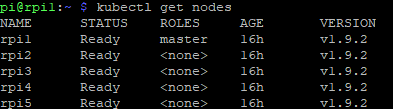
Figure 27: Status query in the terminal of all nodes.
The Kubernetes cluster now has an active master node. If this node ever fails, the kube-controller-manager (see Google Kubernetes) detects this and decides which of the worker nodes will step in as the new active master.
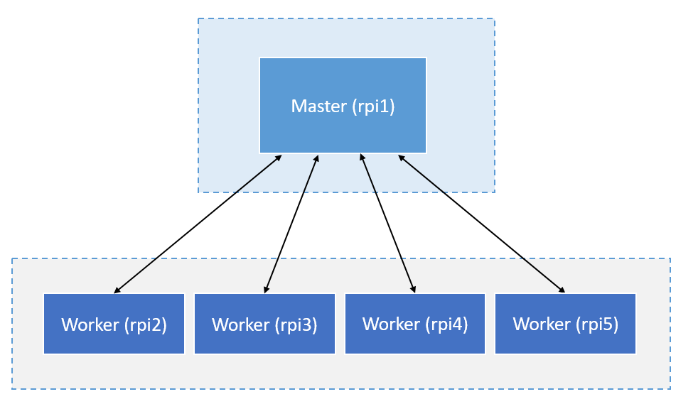
Figure 28: Schematic structure of Kubernetes on the PiCube cluster.
Configuration LCD display
In order for the LCD display to show the corresponding values IP addresses, system time, temperature and status information, a corresponding Python script is used. This script is executed automatically at every startup and delivers status values to the LCD display via I2C. 58
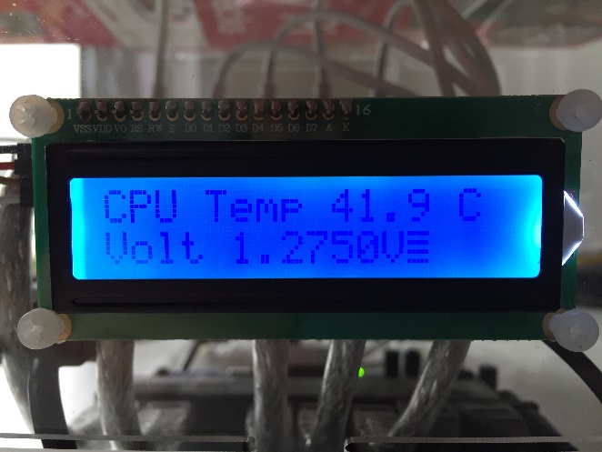
Figure 29a: Display of temperature, voltage and load on the LCD display.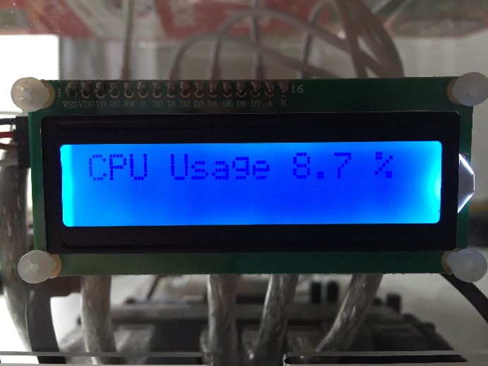
Figure 29b: Display of temperature, voltage and load on the LCD display.
Evaluation
After the cluster has been configured and Kubernetes is ready for use, the entire system is evaluated. The requirements set in advance (see Requirements) are critically reviewed, target and actual values are evaluated, and various comparisons are made. This prototype is ideally suited to illustrate and substantiate the research question addressed in this thesis. Section Use case SETI@home deals with a use case that provides information about the extent to which and the purpose for which this custom cluster construction can contribute to scientific research.
Scalability
Kubernetes enables easy scaling of applications or pods and the applications within them. Enabled autoscaling scales pods according to their required resources up to a specified limit. In the following example, we test the autoscaling of our cluster using a simple web application and verify the automatic scalability of the system: 59
For this purpose, a Docker image based on a simple web server application is used. This Docker image contains a single web page, which causes a maximum CPU load by simulated users when called. The Docker image is launched, causing a web server to run with the corresponding web page as a pod. Kubernetes' autoscaler is enabled with the following configuration: 60
-
KUBE_AUTOSCALER_MIN_NODES = 1: The minimum number of nodes to be used is one.
-
KUBE_AUTOSCALER_MAX_NODES = 4: The maximum number of nodes to be used is four. The fifth node thus retains the function as master.
-
KUBE_ENABLE_CLUSTER_AUTOSCALER = true: Activation of the autoscaler.
The pod with the web server container is started with the following properties:
-
CPU-PERCENT = 50: This configuration value specifies the value that is maintained to keep all pods at an average CPU load of 50 percent.
-
As soon as a pod requires more than half of its available computing power, another pod instance is automatically replicated or an exact copy of the running pod is created.
-
MIN = 1: At least one Pod is used for scaling.
-
MAX = 10: A maximum of ten replicas of a pod can be used for scaling.
After the pod is started and user load is simulated, an increase in CPU load to 250 percent is observed and that seven pods have already been swapped out or scaled:
|
|
Listing 5: Observing CPU utilization increase to 250% while pods are swapped out to provide resources.
Two minutes after the user load simulation stops, the CPU utilization drops back to zero and the drop from seven to one pod can be seen.
|
|
Listing 6: Watching CPU utilization drop to zero percent and drop to one pod.
As can be seen (see Listing 1), it is very easy to dynamically adjust the number of pods to the load, by enabling the cluster autoscaler.
Automatic and dynamic scaling can also be very helpful when there are irregularities in cluster utilization. For example, development-related clusters or continuous computing operations can be run on weekends or at night. Compute-intensive applications can be better scheduled so that a cluster is optimally utilized. In all cases, the cluster can be used optimally. Either reduce the number of unused nodes to save energy or scale to the limit to provide enough computing power. Depending on which case occurs, a dynamically scaling cluster ensures that at high or low utilization, all tasks are solved in the most efficient way.
Fail-safe
As with each element of our cluster, we ensure that more than one instance of each component is running simultaneously. Setting the number to five physical nodes per enclosure is one reason for creating the possibility of optimal scaling and appropriate resilience. The greater the number of nodes, the less likely there is to be a total failure or bottleneck in scaling capabilities. Load balancing and availability are closely related to cluster resilience. One way to ensure that a master node is highly available is to allow a worker node to step in as master. Kubernetes already inherently brings the function that as soon as a master node fails, a worker takes its place. The active/passive design is already in use. Second, this failover implementation is active for all worker nodes. Figure 28 shows how load balancing and failover work together to keep this cluster alive in the event of a master as well as worker node failure. The actors here are the cluster components etcd, kube-apiserver, kube-controller and kube-scheduler (see Google Kubernetes). The Kubernetes API server, controller, and scheduler all run inside Kubernetes as pods. This means that in the event of a failure, each of these pods will be moved to a different node, thus preserving the core services of the cluster. Here, one considers potential failure scenarios:
-
Loss of the master node: If not configured for HA, loss of the master node or its services will have a severe impact on the application. The cluster will not be able to respond to commands or deploy nodes. Each service in the master node is critical and is configured appropriately for HA, so a worker node automatically steps in as the master.
-
Loss of worker nodes: Kubernetes is able to automatically detect and repair pods. Depending on how the services are balanced, there may be an impact on the end users of the application. If any pods on a node are not responding, kubelet detects this and informs the master to use a different pod.
-
Network failure: The master and worker nodes in a Kubernetes cluster can become unreachable due to network failures. In some cases, they are treated as node failures. In this case, other nodes are used accordingly to replace the respective node that is unreachable.
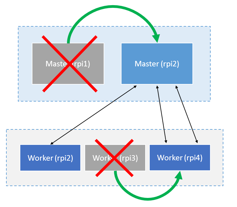
Figure 30: Failure and takeoverscenario of the master node rpi1 and the worker node rpi3.
Kubernetes is configured to be highly available to tolerate the failure of one or more master nodes and up to four worker nodes. This is critical for running development or production environments in Kubernetes. An odd number of nodes is chosen so that it is possible to keep the cluster alive even with only one node. A cluster node can continue to operate in the last instance once a node is only acting as a master and worker. In this state, the cluster is neither highly available, fail-safe, nor completely resilient, but it survives.
Cost efficiency and performance
Looking at the costs, there are two sides to the story. With the total acquisition costs, minus the contributed effort to assemble, install and configure the cluster, the value of the investment is exactly 358.79 EUR. This construct is contrasted with a simple Linux cluster for comparison. This Linux cluster consists of commercially available PCs with comparable core data to that of the Raspberry Pi nodes.
| Raspberry Pi 3 Model B | Linux PC | |
|---|---|---|
| CPU | Cortex-A53 1.2 GHz Quadcore | Intel Celeron J1900 2 GHz Quadcore |
| RAM | 1024 MB | 4 GB RAM |
| Network | 100 Mbps | 1000 Mbps |
| Current Consumption | max. 4 Watt / h | max. 10 Watt / h |
| Price per computer | approx. 35 € | approx. 95 € |
| Total price | approx. 175 € | approx. 475 € |
Table 2: Cost comparison of the core components of Raspberry Pi and Linux PC.
If we now compare the core data, we can see that the comparison system is definitely associated with higher acquisition costs. It is important to mention that this comparison primarily focuses on the costs and not the performance of the individual systems. It is obvious that a Linux PC, based on a CISC processor architecture, definitely achieves higher FLOPS than an ordinary ARM processor. Nevertheless, it becomes clear in the first approach that, despite the lower performance, there is a significant difference in terms of cost. Especially when performance per watt is calculated. Due to the compact design of the Raspberry Pi and the accommodation of all components, such as the integrated power supply and GPU, it is a competitive partner for the Linux PC.
In relation to the costs, the question arises how the comparison systems perform in terms of performance. For this, a performance test is performed with the help of sysbench. Sysbench is a benchmark application that quickly gives an impression of the system performance. For this purpose, a CPU benchmark is run on both systems, which calculates all prime numbers up to 20000, and the results are shown in Table 3 and Figure 31.
| Raspberry Pi 3 Model B | Linux PC | |
|---|---|---|
| CPU benchmark | Prime number calulation | Prime number calculation |
| Threads (process parts) | 4 | 4 |
| Limit | 20000 | 20000 |
| Calculation time | 115.1536 seconds | 11.2800 seconds |
Table 3: Comparison times of the prime number calculation up to 20000.
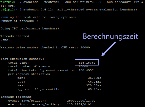
Figure 31: Results of the sysbench benchmark run on node rpi2.
The difference in the calculation time is clearly visible. There is a difference of 104 seconds. According to the visible comparisons and as already mentioned in the cost comparison, there is no question that a Linux PC based on the CISC architecture has a higher CPU performance than the Raspberry Pi with an ARM architecture.
Energy efficiency and cooling
ARM processors, such as those installed on the Raspberry Pi, have a high energy efficiency with a clock frequency of 1.2 GHz and a power consumption of max. 4 watts. The average power consumption is about 2 watts in idle mode. The switch consumes 2.4 watts at 0.2 amps of current and 12 volts. The total wattage output of the USB charger is made up of all components and sits at the end of the power chain. Summarizing with all installed components, you get a total power consumption of 13.75 watts in idle and 34 watts at maximum load (see Table 4).
| Power consumption | ||
|---|---|---|
| Component | Idle | maximum |
| Raspberry Pi 3 Model B | 2 Watt | 4 Watt |
| Edimax ES-5800G V2 Gigabit Switch (8-Port) | 2.4 watt | 2.4 watt |
| LCD display module 1602 HD44780 with TWI controller | 0.1 watt | 0.1 watt |
| Antec TRICOOL 92mm 4-pin case fan | 1.25 watt | 1.25 watt |
| Anear 60 Watt USB Charger (6-Port) | - | - |
| Total power consumption | 13,75 Watt | 23,75 Watt |
Table 4: Total power consumption of the PiCube in idle mode and maximum CPU load of 100%.
In the following test, CPU load is generated using the Sysbench prime calculation program and advantages and disadvantages are shown by using active cooling and passive cooling elements. We read system values such as temperature, clock frequency and voltage using the following commands in each case: 61
|
|
Listing 7: Commands for querying temperature, clock frequency and voltage.
In the following, we look at three temperature curves in the case. The CPU clock frequency is 1.2 GHz and the CPU voltage is 1.325 volts over a period of 5 minutes:
- Temp1: In case, without heatsink on SoC, without active cooling.
- Temp2: In case, with heatsink on SoC, without active cooling.
- Temp3: In case, with heatsink on SoC, with active cooling.
| **CPU utilization (%) | Temp1 (°C) | Temp2 (°C) | Temp3 (°C) |
|---|---|---|---|
| 0 | 39 | 39 | 44 |
| 100 | 77 | 77 | 82 |
Table 5: Measured values of heat generation without active cooling.
Next, we look at three temperature profiles of a Raspberry Pi processor. The CPU clock frequency is 1.2 GHz and the CPU voltage is 1.325 volts over a period of 10 minutes:
- Temp1: CPU, without heat sink on SoC, without active cooling.
- Temp2: CPU, with heat sink on SoC, without active cooling.
- Temp3: CPU, with heat sink on SoC, with active cooling.

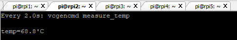
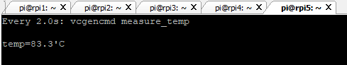
| **CPU utilization (%) | Temp1 (°C) | Temp2 (°C) | Temp3 (°C) |
|---|---|---|---|
| 0 | 44 | 32,2 | 27,8 |
| 100 | 83,3 | 83,3 | 69,8 |
Table 6: Measured values
The heat development of the circuit boards of each individual computer is also taken into account. Although this is low, it increases constantly with the number of nodes installed in the case. The heat development is about 35 degrees Celsius with an average load of a single board. With 5 nodes, this is already around 38 degrees, which corresponds to a factor of around 1.08 per node. If all 5 nodes are overclocked by increasing the processor's clock frequency, this factor increases to 1.1. Temperature differences of 10 degrees in the case and the processor prove that the maximum performance of all hardware nodes cannot be exploited without appropriate cooling. Passive heat sinks and an already implemented active cooling with the help of a case fan can help here. There is no question that the optimized airflow inside the case also contributes to the improved cooling performance.
Use Case SETI@home
After evaluating the cluster, we turn to a use case from the scientific domain. A current PRC project of BOINC is SETI@home, a scientific experiment run by the University of California at Berkeley that uses computers connected to the Internet in the search for extraterrestrial intelligence. One participates by running a free client program on a computer that downloads and analyzes radio telescope data. This project relies on the concept of grid computing. Data sets to be processed are divided into smaller data sets and distributed to all participating clients, who compute and communicate the results to the distributor, which reassembles the computations into an overall data set. The current computing power of the entire BOINC grid is 20600 PetaFLOPS, distributed over nearly 0.9 million computers. SETI@home has a share of about 19.1% of this. 62
In the following, container virtualization is exploited and pre-built BOINC client images of Docker are used. These images are prefabricated containers, which are started as scalable pods on the PiCube and scale automatically in order to utilize the entire computing power of the cluster. To do this, you register with the SETI@home project and create an account. Using this account data, you generate a container application called k8s-boinc-demo and start it on the cluster with a scaling limit of 10 pod instances. In Figure 32, you can see from the Kubernetes dashboard how the pods are distributed evenly or according to workload across worker nodes rpi2 to rpi5 after launch. 63
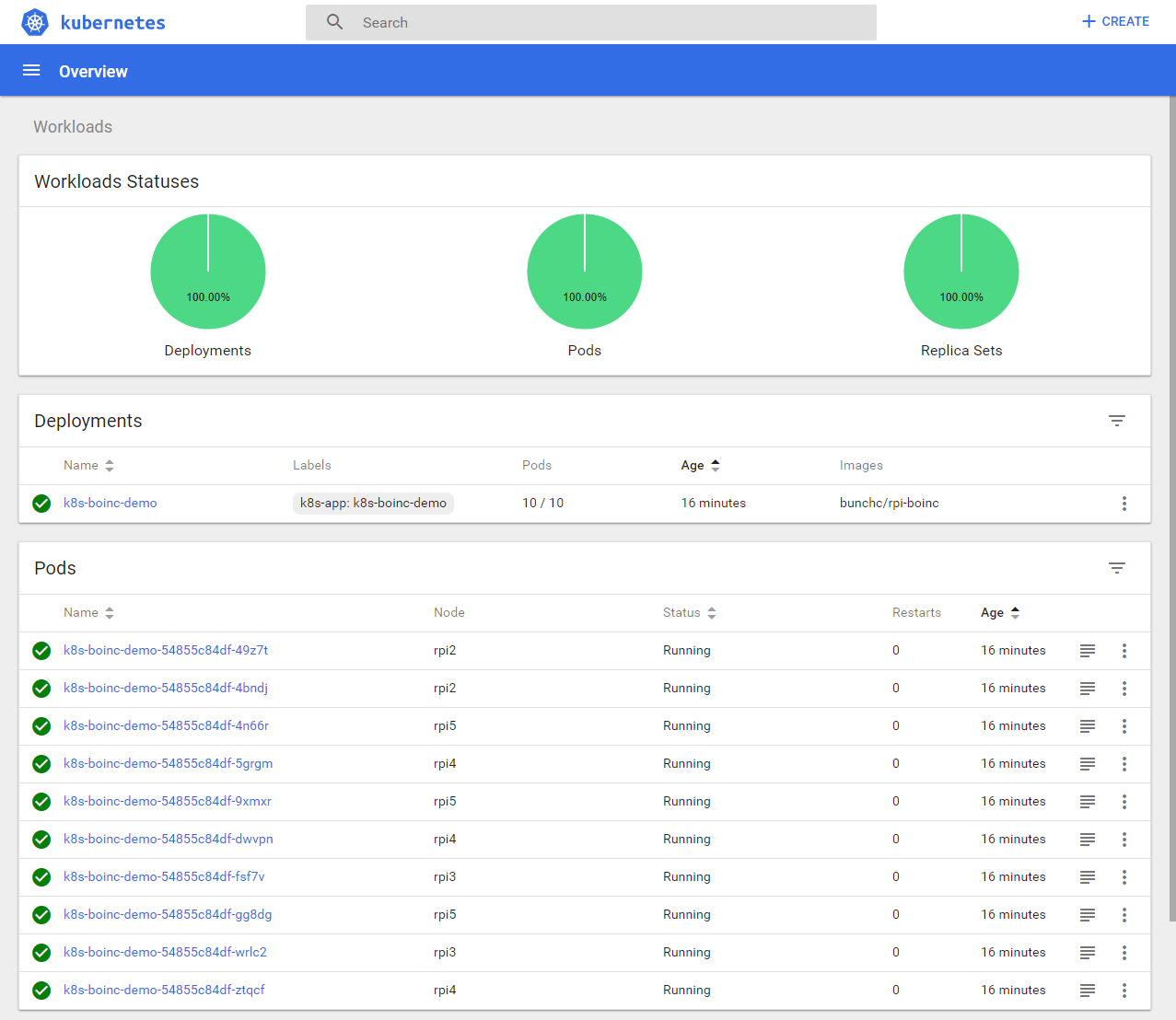
Figure 32: Overview of the utilization, status and distribution of the pods on the nodes rpi2 to rpi5.
Within the SETI@home account, we define how the individual clients or pods are utilized. The CPU utilization is left at the default value of 100% and after about 5 minutes you can see how the CPU utilization of all cluster nodes increases to 100% and remains constant at this value (see Figure 33). The cluster now computes data of the SETI@home project.
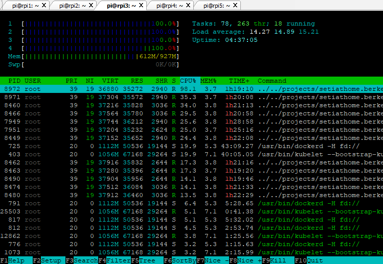
Figure 33: The CPU utilization of node rpi3 at 100%.
Figure 33 shows the computers currently logged in to the grid with our account information. Each pod is identified here as a single client. If we now assume that the number of PiCube clusters increases to ten, the number of pods would multiply by the same factor. With 10 pod instances per cluster, this means 100 active SETI@home clients, which could make their computing power available to the BOINC grid.
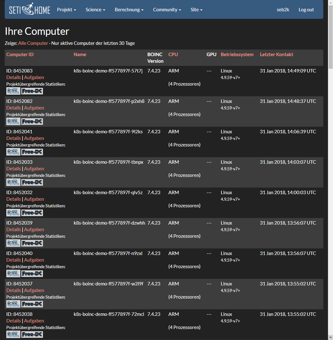
Figure 34: Listing of all logged-in clients or pods in our cluster.
As this use case shows, it can be inferred that the scientific utility of this cluster is without question. Using dynamic pod scaling, it is demonstrated that even when individual nodes have low performance, they can achieve high computing performance when combined as a swarm. BOINC's computing grid is a typical example of how computers, distributed around the world and connected via the Internet, can solve problems together.
Conclusion and outlook
It is possible to construct a comparable system of a supercomputer with low costs. It is obvious that the performance of an ARM processor cannot currently keep up with commercially available CISC processors, as described in Cost efficiency and performance. However, the use case and illustration of dynamic scaling show that once distributed systems are interconnected, they develop very high parallel computing power. The Raspberry Pi cluster provides an interesting approach to perform tests or use cases in research, education, and academia. ARM architectures are evolving rapidly in terms of performance and efficiency over the next few years, with power consumption always in mind. The requirements set at the beginning of this thesis, such as energy efficiency, resilience and modularity, have been met and sensibly implemented in the construct. There is no question that this PiCube cluster is not a real competitor to massively parallelized supercomputers, but the decisive approach lies in the benefit of a computing grid.
There are several ways to use this system in the future. On the one hand, its simplicity means it can be used for cluster computing to provide a small, full-featured, low-cost, energy-efficient development platform. This includes understanding its limitations in terms of performance, usability and maintainability. On the other hand, it can act as a mobile and self-sufficient cloud in a box system by adding components such as solar cells and mobile connectivity. Either way, it will remain a fascinating project that offers developers many possibilities and gives a think-out-of-the-box approach.
Bibliography
Adams, J. (September 2017). SFT Guide 14/17 - Raspberry Pi Tips, Tricks & Hacks (No. 1). Third generation: The innovations of the Raspberry Pi 3, p. 159.
Baier, J. (2017). Getting Started with Kubernetes - Harness the power of Kubernetes to manage Docker deployments with ease. Birmingham: Packt Publishing.
Bauke, H., & Mertens, S. (2006). Cluster computing - Practical introduction to high performance computing on Linux clusters. Heidelberg: Springer.
Bedner, M. (2012). Cloud computing - technology, security and legal design. Kassel: kassel university press.
Bengel, G., Baun, C., Kunze, M., & Stucky, K.-U. (2008). Master course parallel and distributed systems - fundamentals and programming of multicore processors, multiprocessors, clusters and grids. Wiesbaden: Vieweg+Teubner.
Beowulf Cluster Computing. (January 12, 2018). Retrieved from MichiganTech - Beowulf Cluster Computing: http://www.cs.mtu.edu/beowulf/
Beowulf Scalable Mass Storage (T-Racks). (January 12, 2018). Retrieved from ESS Project: https://www.hq.nasa.gov/hpcc/reports/annrpt97/accomps/ess/WW80.html
BOINC - Active Projects Statistics. (January 31, 2018). Retrieved from Free-DC - Distributed Computing Stats System: http://stats.free-dc.org/stats.php?page=userbycpid&cpid=cfbdd0ffc5596f8c5fed01bbe619679d
Cache.(January 14, 2018). Retrieved from Electronics Compendium: https://www.elektronik-kompendium.de/sites/com/0309291.htm
Christl, D.,Riedel, M., & Zelend, M. (2007). Communication systems / computer networks - Research of tools for the control of a massively parallel cluster computer in the computer center of the West Saxon University of Applied Sciences Zwickau. Zwickau: Westsächsichen Hochschule Zwickau.
CISC and RISC. (January 28, 2018). Retrieved from Electronics Compendium: https://www.elektronik-kompendium.de/sites/com/0412281.htm
Containersvs. virtual machines. (December 13, 2017). Retrieved from NetApp Blog: https://blog.netapp.com/blogs/containers-vs-vms/
Coulouris, G.,Dollimore, J., Kindberg, T., & Blair, G. (2012). Distributed systems - concepts and design. Boston: Pearson.
Dennis, A. K. (2013). Raspberry Pi super cluster. Birmingham: Packt Publishing.
The science behind SETI@home. (January 30, 2018). Retrieved from SETI@home: https://setiathome.berkeley.edu/sah_about.php
Docker on the Raspberry Pi with HypriotOS. (January 24, 2018). Retrieved from Raspberry Pi Geek: http://www.raspberry-pi-geek.de/Magazin/2017/12/Docker-auf-dem-Raspberry-Pi-mit-HypriotOS
Eder,M. (2016). Hypervisor- vs. container-based virtualization. Munich: Technical University of Munich.
Einstein@Home on Android devices. (January 23, 2018). Retrieved from GEO600: http://www.geo600.org/1282133/Einstein_Home_on_Android_devices
Enable I2C Interface on the Raspberry Pi. (January 28, 2018). Retrieved from Raspberry Pi Spy: https://www.raspberrypi-spy.co.uk/2014/11/enabling-the-i2c-interface-on-the-raspberry-pi/
Encyclopedia - VAX. (January 20, 2018). Retrieved from PCmag: https://www.pcmag.com/encyclopedia/term/53678/vax
Failover Cluster. (January 20, 2018). Retrieved from Microsoft Developer Network: https://msdn.microsoft.com/en-us/library/ff650328.aspx
Fenner, P. (10. 12 2017). So What's a Practical Laser-Cut Clip Size? Retrieved from DefProc Engineering: https://www.deferredprocrastination.co.uk/blog/2013/so-whats-a-practical-laser-cut-clip-size/Fey, D. (2010).
Grid computing - An enabling technology for computational science. Heidelberg: Springer.
GitHub - flash. (January 24, 2018). Retrieved from hypriot / flash: https://github.com/hypriot/flash
Goasguen, S. (2015). Docker Cookbook - Solutions and Examples for Building Dsitributed Applications. Sebastopol: O'Reilly.
Grabsch, V., & Radunz, Y. (2008). Seminar presentation - Amdahl's and Gustafson's law. o.O.: Creative Commons.
Herminghaus, V., & Scriba, A. (2006). Veritas Storage Foundation - High End Computing for UNIX Design and Implementation of High Availability Solutions with VxVM and VCS. Heidelberg: Springer.
Horizontal Pod Autoscaling. (January 29, 2018). Retrieved from GitHub: https://github.com/kubernetes/kubernetes/blob/8caeec429ee1d2a9df7b7a41b21c626346b456fb/docs/user-guide/horizontal-pod-autoscaling/image/index.php
How nodes work. (January 27, 2018). Retrieved from docker docs: https://docs.docker.com/engine/swarm/how-swarm-mode-works/nodes/
How to setup an I2C LCD on the Raspberry Pi. (January 28, 2018). Retrieved from Circuit Basics: http://www.circuitbasics.com/raspberry-pi-i2c-lcd-set-up-and-programming/
If we want to Find Aliens, We Need to Save the Arecibo Telescope. (January 23, 2018). Retrieved from vice: https://www.vice.com/en_us/article/wdbq74/find-aliens-arecibo-telescope
Inkscape - Overview. (January 24, 2018). Retrieved from Inkscape: https://inkscape.org/de/ueber/uebersicht/
Kaiser, R. (2009). Virtualization of multiprocessor systems with real-time applications. Koblenz-Landau.Kersken, S. (2015).
IT handbook for IT specialists. Bonn: Rheinwerk Verlag GmbH.
Kroeker, K. L. (March 2011). Grid computing's future. Communications of the ACM, pp. 15-17.
Kubernetes Components. (January 10, 2018). Retrieved from kubernetes: https://kubernetes.io/docs/concepts/overview/components/
Kubernetes vs Docker Swarm. (January 10, 2018). Retrieved from Platform9: https://platform9.com/blog/kubernetes-docker-swarm-compared/
Laser-Cut Elastic-Clipped Comb-Joints. (December 1, 2018). Retrieved from DefProc Engineering: https://www.deferredprocrastination.co.uk/blog/2013/laser-cut-elastic-clipped-comb-joints/
Laser-Cut Elastic Clips. (December 1, 2017). Retrieved from Thingiverse: https://www.thingiverse.com/thing:53032
Lee, C. (2014). Cloud database development and management. Boca Raton: CRC Press.
Liebel, O. (2011). Linux high availability - deployment scenarios and practical solutions. Bonn: Galileo Press.
Load-Balanced Cluster. (January 20, 2018). Retrieved from Microsoft Developer Network: https://msdn.microsoft.com/en-us/library/ff648960.aspx
Lobel, L. G., & Boyd, E. D.. (2014). Microsoft Azure SQL Database step by step. Redmond: Microsoft Press.
MAD - Andreas Gregori. (January 24, 2018). Retrieved from MAD Models Architecture Design: http://mad-modelle.de/kontakt/
Mandl, P. (2010). Basic course operating systems - architectures, resource management, synchronization, process communication. Wiesbaden: VIeweg + Teubner.
Matros, R. (2012). The impact of cloud computing on IT service providers - A case study-based investigation of critical influencing variables. Bayreuth: Springer
Gabler.Merkert, J. (16 October 2017). c't Raspberry Pi - Raspi projects. Risc OS, p. 151.
Miell, I., & Sayers, A. H. (2016). Docker in practice. New York: Manning Publications.
Networked computing: fundamentals and applications. (January 20, 2018). Retrieved from techchannel: https://www.tecchannel.de/a/networked-computing-grundlagen-und-anwendungen,439222,5
Neuenschwander, E. P. (2014). Cloud computing - A legal thundercloud? Zurich: University of Zurich.
New DIY supercomputer saves £1,000s. (January 8, 2018). Retrieved from University of Westminster: https://www.westminster.ac.uk/news-and-events/news/2011/new-diy-supercomputer-saves-%C2%A31000s
Nickoloff, J. (2016). Docker in action. New York: Manning Publications.
Nodes. (January 10, 2018). Retrieved from kubernetes: https://kubernetes.io/docs/concepts/workloads/pods/pod-overview/
Overview of Microsoft HPC Pack and SOA in Failover Cluster. (January 21, 2018). Retrieved from Microsoft TechNet: https://technet.microsoft.com/en-us/library/gg142067(v=ws.11).aspx
PaaS or IaaS. (January 13, 2018). Retrieved from Microsoft Azure: https://docs.microsoft.com/de-de/azure/sql-database/sql-database-paas-vs-sql-server-iaas
Parallel Linux Operating System - Beowulf Gigaflop/s Workstation Project. (January 12, 2018). Retrieved from ESS Project: https://www.hq.nasa.gov/hpcc/reports/annrpt97/accomps/ess/WW49.html
Pfister, G. (1997). In Search of Clusters - The ongoing Battle in lowly Parallel Computing. New Jersey: Prentice Hall.
Pods. (January 10, 2018). Retrieved from kubernetes: https://kubernetes.io/docs/concepts/workloads/pods/pod-overview/
Pods and Nodes. (January 10, 2018). Retrieved from kubernetes Bootcamp: https://kubernetesbootcamp.github.io/kubernetes-bootcamp/3-1.html
Project list. (January 8, 2018). Retrieved from BOINC: http://boinc.berkeley.edu/wiki/Project_list
Project to setup Boinc client in Docker for the RaspberryPi. (January 30, 2018). Retrieved from Docker Hub: https://hub.docker.com/r/bunchc/rpi-boinc/
projects. (November 30, 2017). Retrieved from Climbers.net: http://climbers.net/sbc/diy-raspberry-pi-3-cluster/RPiCluster4b.png
Raspberry Pi 3 - self-heating. (Dec 20, 2017). Retrieved from mikrocontroller.net: https://www.mikrocontroller.net/topic/393898
Raspberry Pi 3 GPIO Pin Chart with Pi. (January 23, 2018). Retrieved from openclipart: https://openclipart.org/detail/280972/raspberry-pi-3-gpio-pin-chart-with-pi
Raspberry Pi 3: Power consumption and CoreMark comparison. (January 31, 2018). Retrieved from heise online: https://www.heise.de/ct/artikel/Raspberry-Pi-3-Leistungsaufnahme-und-CoreMark-Vergleich-3121139.html
Ries, C. B. (2012). BOINC - high performance computing with Berkeley Open Infrastructure for Network Computing. Heidelberg: Springer Vieweg.
rkt - A security-minded, standards-based container engine. (January 27, 2018). Retrieved from CoreOS: https://coreos.com/rkt/
RPiCluster - Overview. (January 23, 2018). Retrieved from RPiCluster: https://bitbucket.org/jkiepert/rpicluster
Schill, A., & Springer, T. (2007). Distributed systems - fundamentals and enabling technologies. Heidelberg: Springer.
SETI@home - Your Computers. (January 31, 2018). Retrieved from SETI@home: https://setiathome.berkeley.edu/hosts_user.php
Smith, N. (28. 11 2017). Climbers.net. Retrieved from DIY 5 Node Cluster of Raspberry Pi 3s: http://climbers.net/sbc/diy-raspberry-pi-3-cluster/
Swarm mode key concepts. (January 27, 2018). Retrieved from docker docs: https://docs.docker.com/engine/swarm/key-concepts/
Tanenbaum, A. S. (2007). Distributed systems - principles and paradigms. New Jersey: Pearson Prentice Hall.
Technet. (January 13, 2018). Retrieved from Microsoft: https://blogs.technet.microsoft.com/kevinremde/2011/04/03/saas-paas-and-iaas-oh-my-cloudy-april-part-3/
Top500 List. (January 8, 2018). Retrieved from Top 500 The List: https://www.top500.org/list/2017/11/
Ulmann, B. (February 6, 2014). IT basics. FOM.
Our home galaxy - the Milky Way. (January 23, 2018). Retrieved from planet wissen: https://www.planet-wissen.de/technik/weltraumforschung/astronomie/pwieunsereheimatgalaxiediemilchstrasse100.html
VMS Software, Inc. Named Exclusive Developer of Future Versions of OpenVMS Operating System. (January 20, 2018). Retrieved from BusinessWire: https://www.businesswire.com/news/home/20140731006118/en/VMS-Software-Named-Exclusive-Developer-Future-Versions
What is Kubernetes? (January 10, 2018). Retrieved from kubernetes: https://kubernetes.io/docs/concepts/overview/what-is-kubernetes/
Appendix A - Script: Installing Kubernetes
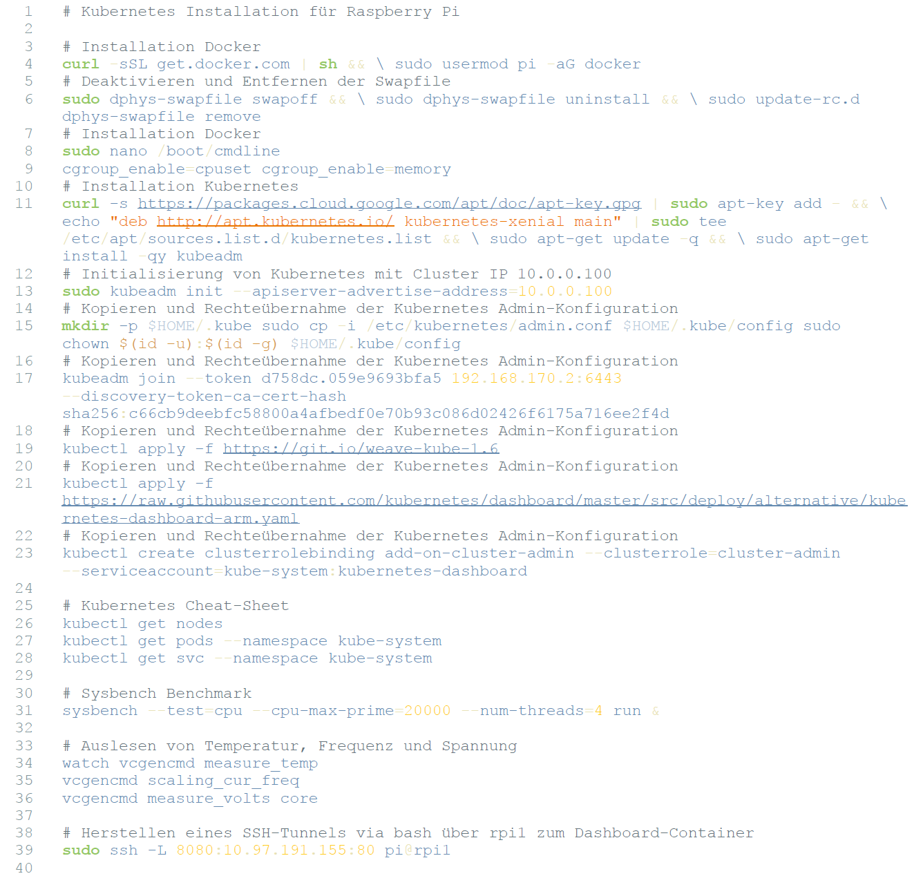
Appendix B - Script: LCD display
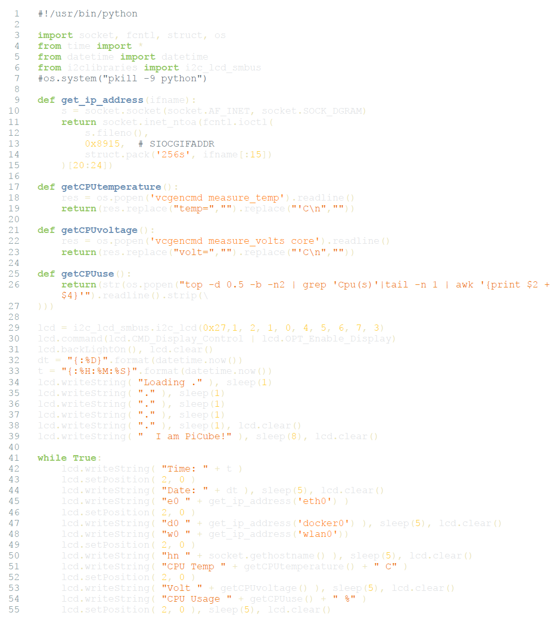
Appendix C - Script: Docker Autoscaling
Dockerfile:
|
|
index.php:
|
|
-
Cf. (Grabsch & Radunz, 2008, p. 2ff) ; (Kaiser, 2009, p. 16f). ↩︎
-
Cf. (Bengel, Baun, Kunze, & Stucky, 2008, p. 319f) ; (Grabsch & Radunz, 2008, pp. 7-11) ↩︎
-
Cf. ibid. ↩︎
-
Cf. (Kersken, 2015, p. 197). ↩︎
-
Cf. (Bengel, Baun, Kunze, & Stucky, 2008, p. 2) ; (Kersken, 2015, p. 198ff). ↩︎
-
Cf. (Bengel, Baun, Kunze, & Stucky, 2008, p. 2f) ; (Schill & Springer, 2007, p. 31). ↩︎
-
Cf. ibid. ↩︎
-
Cf. (Bengel, Baun, Kunze, & Stucky, 2008, p. 435) ; (Fey, 2010, p.
- ; (Tanenbaum, 2007, p. 18f).
-
Cf. (Liebel, 2011, p. 171) ; (Bengel, Baun, Kunze, & Stucky, 2008, pp. 3, 435) ; Cf. (Fey, 2010, p. 5). ↩︎
-
Cf. (Schill & Springer, 2007, p. 26f). . ↩︎
-
Cf. (Ries, 2012, p. 17). ↩︎
-
Cf. ibid; (Kroeker, 2011, p. 15). ↩︎
-
Cf. (Project list, 2018) ; (Bauke & Mertens, 2006, pp. 32-34) ; (Our home galaxy - the Milky Way, 2018) ; (If we want to Find Aliens, We Need to Save the Arecibo Telescope, 2018) ; (Einstein@Home on Android Devices, 2018). ↩︎
-
Cf. (New DIY supercomputer saves £1,000s, 2018). ↩︎
-
Cf. (Tanenbaum, 2007, p. 2) ; (Bengel, Baun, Kunze, & Stucky, 2008, p. 26). ↩︎
-
Cf. (Coulouris, Dollimore, Kindberg, & Blair, 2012, p. 2) ; (Tanenbaum, 2007, p. 9) ; (Coulouris, Dollimore, Kindberg, & Blair, 2012, pp. 2, 598f, 603f) ; (Tanenbaum, 2007, pp. 232, 240). ↩︎
-
Cf. (Coulouris, Dollimore, Kindberg, & Blair, 2012, pp. 125, 128, 464). ↩︎
-
Cf. (Bedner, 2012, p. 6f, 22f) ↩︎
-
Cf. (Coulouris, Dollimore, Kindberg, & Blair, 2012, p. 13f). . ↩︎
-
Cf. (Matros, 2012, p. 139) ; (Lee, 2014, p. 8ff) ; (Lobel & Boyd, 2014, p. 3f). ↩︎
-
Cf. (Neuenschwander, 2014, p. 4) ; (Bedner, 2012, p. 32ff) ; (PaaS or IaaS, 2018). ↩︎
-
Cf. (Bauke & Mertens, 2006, p. 51). ↩︎
-
(Pfister, 1997, p. 98). ↩︎
-
Cf. (Liebel, 2011, p. 169ff) ; (Schill & Springer, 2007, p. 24ff) ; (Bengel, Baun, Kunze, & Stucky, 2008, p. 415). ↩︎
-
Cf. (Top500 List, 2018) ; (Liebel, 2011, p. 169ff) ; (Schill & Springer, 2007, p. 24ff). ↩︎
-
Cf. (Ulmann, 2014, p. 51f) ; (Bauke & Mertens, 2006, p. 21). ↩︎
-
Cf. (Cache, 2018) ; (Bauke & Mertens, 2006, p. 21f) ; (Christl, Riedel, & Zelend, 2007, p. 5). ↩︎
-
Cf. (Bauke & Mertens, 2006, p. 22ff) ; (Christl, Riedel, & Zelend, 2007, p. 5). ↩︎
-
Cf. (Ries, 2012, p. 11) ; (Bengel, Baun, Kunze, & Stucky, 2008, pp. 190f, 205) ; (Dennis, 2013, p. 41f) ; (Bauke & Mertens, 2006, pp. 143ff, 45). ↩︎
-
Cf. (Liebel, 2011, p. 170f) ; (Failover Cluster, 2018). ↩︎
-
Cf. (Failover Cluster, 2018) ; (Liebel, 2011, p. 185f). ↩︎
-
Cf. (Christl, Riedel, & Zelend, 2007) ; (Bauke & Mertens, 2006, p. 52f). ↩︎
-
Cf. (Bauke & Mertens, 2006, p. 51f) ; (Christl, Riedel, & Zelend, 2007, p. 4) ; (Overview of Microsoft HPC Pack and SOA in Failover Cluster, 2018). ↩︎
-
Cf. (VMS Software, Inc. Named Exclusive Developer of Future Versions of OpenVMS Operating System., 2018) ; (Encyclopedia - VAX, 2018). ↩︎
-
Cf. (Load-Balanced Cluster, 2018). ↩︎
-
Cf. (Beowulf Cluster Computing, 2018) ; (Parallel Linux Operating System - Beowulf Gigaflop/s Workstation Project, 2018) ; (Beowulf Scalable Mass Storage (T-Racks), 2018). ↩︎
-
Cf. (Christl, Riedel, & Zelend, 2007, p. 9f). . ↩︎
-
Cf. (Bauke & Mertens, 2006, p. 9, 27f) ; (Kersken, 2015, p. 126) . ↩︎
-
Cf. (Coulouris, Dollimore, Kindberg, & Blair, 2012, p. 318f). . ↩︎
-
Cf. (Kaiser, 2009, p. 41, 43) ; (Mandl, 2010, p. 28f) ; (Eder, 2016, p. 1f). ↩︎
-
Cf. (Eder, 2016, p. 1ff). ↩︎
-
Cf. (rkt - A security-minded, standards-based container engine, 2018). ↩︎
-
Cf. (Nickoloff, 2016, p. 4f) ; (Goasguen, 2015, p. 1) ; (Miell & Sayers, 2016, p. 5f) ; (How nodes work, 2018) ↩︎
-
Cf. (Nickoloff, 2016, p. 255) ; (Goasguen, 2015, p. 199) ; (Swarm mode key concepts, 2018) ↩︎
-
Cf. (Nickoloff, 2016, p. 255) ; (Goasguen, 2015, p. 199) ; (Swarm mode key concepts, 2018). ↩︎
-
Cf. (What is Kubernetes?, 2018). ↩︎
-
Cf. (Nodes, 2018) ; (Pods, 2018). ↩︎
-
Cf. (Kubernetes Components, 2018). ↩︎
-
Cf. ibid. ↩︎
-
Cf. (CISC and RISC, 2018) ; (Ulmann, 2014, p. 71) ; (Merkert, 2017, p. 20) ; (Adams, 2017, p. 8). ↩︎
-
Cf. (Adams, 2017, p. 7). ↩︎
-
Cf. (Smith, 2017) ; (RPiCluster - Overview, 2018). ↩︎
-
Cf. (Laser-Cut Elastic-Clipped Comb-Joints, 2018). ↩︎
-
Cf. (Fenner, 2017). ↩︎
-
(Inkscape - Overview, 2018) ↩︎
-
Cf. (Docker on the Raspberry Pi with HypriotOS, 2018). . ↩︎
-
Cf. (GitHub - flash, 2018). ↩︎
-
Cf. (Enable I2C Interface on the Raspberry Pi, 2018) ; (How to setup an I2C LCD on the Raspberry Pi, 2018). ↩︎
-
Cf. (Horizontal Pod Autoscaling, 2018). ↩︎
-
Cf. (Baier, 2017, p. 117). ↩︎
-
Cf. (Raspberry Pi 3: Power consumption and CoreMark comparison, 2018). . ↩︎
-
Cf. (The Science Behind SETI@home, 2018) ; Cf. (BOINC - Active Projects Statistics, 2018) ↩︎
-
Cf. (Project to setup Boinc client in Docker for the RaspberryPi, 2018). ↩︎